The essence of the simulation method. Simulation of economic processes: characteristics and main types
Read also
FEDERAL FISHERIES AGENCY
MINISTRY OF AGRICULTURE
KAMCHATKA STATE TECHNICAL UNIVERSITY
DEPARTMENT OF INFORMATION SYSTEMS
Topic: "IMITATION MODELING OF ECONOMIC
ACTIVITIES OF THE ENTERPRISE "
Course work
Manager: position
Bilchinskaya S.G. "__" ________ 2006
Developer: student gr.
Zhiteneva D.S. 04 Pi1 "__" ________ 2006
The work is protected "___" __________ 2006. with an estimate of ______
Petropavlovsk-Kamchatsky, 2006
Introduction ................................................. .................................................. ......................... 3
1. Theoretical foundations of simulation modeling .......................................... 4
1.1. Modeling. Simulation .......................................... 4
1.2. Monte Carlo method .............................................. ............................................ nine
1.3. Using the laws of distribution of random variables ....................... 12
1.3.1. Uniform distribution ................................................ ................ 12
1.3.2. Discrete distribution (general case) ....................................... 13
1.3.3. Normal distribution................................................ .................. fourteen
1.3.4. Exponential distribution ................................................ ...... 15
1.3.5. Generalized Erlang Distribution ............................................... .. 16
1.3.6. Triangular distribution ................................................ ................. 17
1.4. Planning a simulation computer experiment ................... 18
1.4.1. Cybernetic approach to the organization of experimental research of complex objects and processes ........................................ .................................................. ............. eighteen
1.4.2. Regression analysis and model experiment control. 19
1.4.3. Orthogonal planning of the second order ................................ 20
2. Practical work .............................................. .................................................. ..... 22
3. Conclusions on the Business Model "Production Efficiency" ................................... 26
Conclusion................................................. .................................................. ..................... 31
Bibliography............................................... ................................... 32
APPENDIX A ................................................ .................................................. .......... 33
APPENDIX B ................................................ .................................................. ........... 34
APPENDIX B ................................................ .................................................. ........... 35
APPENDIX D ................................................ .................................................. ........... 36
APPENDIX E ................................................ .................................................. ........... 37
APPENDIX E ................................................ .................................................. ........... 38
INTRODUCTION
Modeling in economics began to be applied long before economics finally took shape as an independent scientific discipline. Mathematical models were used by F. Quesnay (1758 Economic Table), A. Smith (classical macroeconomic model), D. Ricardo (model of international trade). In the 19th century, the mathematical school made a great contribution to modeling (L. Walras, O. Cournot, V Pareto, F. Edgeworth, etc.). In the XX century, the methods of mathematical modeling of the economy were used very widely and their use is associated with the outstanding works of the Nobel Prize laureates in economics (D. Hicks, R. Solow, V. Leontiev, P. Samuelson).
Course work on the subject "Simulation of economic processes" is an independent educational and research work.
The purpose of writing this course work is to consolidate theoretical and practical knowledge. Coverage of approaches and methods of applying simulation modeling in project economic activities.
The main task is to investigate, using simulation modeling, the effectiveness of the economic activity of the enterprise.
1. THEORETICAL BASIS OF SIMULATION
1.1. Modeling. Simulation modeling
In the process of managing various processes, the need to predict the results in certain conditions constantly arises. To speed up the decision to choose the optimal control option and save money for the experiment, process modeling is used.
Modeling is the transfer of the properties of one system, which is called the object of modeling, to another system, which is called the model of the object, the impact on the model is carried out in order to determine the properties of the object by the nature of its behavior.
Such a replacement (transfer) of the properties of an object has to be done in cases where its direct study is difficult or even impossible. As the practice of modeling shows, replacing an object with its model often gives a positive effect.
A model is a representation of an object, system or concept (idea) in some form, different from the form of their real existence. A model of an object can be either an exact copy of this object (albeit made from a different material and on a different scale), or display some of the characteristic properties of an object in an abstract form.
Simultaneously, in the process of modeling, it is possible to obtain reliable information about the object with less time, finances, funds and other resources.
The main goals of modeling are:
1) analysis and determination of properties of objects according to the model;
2) designing new systems and solving optimization problems on the model (finding the best option);
3) management of complex objects and processes;
4) predicting the behavior of an object in the future.
The following types of modeling are most common:
1) mathematical;
2) physical;
3) imitation.
In mathematical modeling, the object under study is replaced by the corresponding mathematical relations, formulas, expressions, with the help of which certain analytical problems are solved (analysis is done), optimal solutions are found, and forecasts are also made.
Physical models are real systems of the same nature as the investigated object, or a different one. The most typical option for physical modeling is the use of mock-ups, installations, or the selection of fragments of an object for conducting limited experiments. And most widely it found application in the natural sciences, sometimes in economics.
For complex systems, which include economic, social, information and other socio-information systems, simulation modeling has found wide application. This is a widespread type of analog modeling, implemented using a set of mathematical tools for special simulating computer programs and programming technologies, which allow, through analogous processes, to conduct a targeted study of the structure and functions of a real complex process in the computer memory in the "simulation" mode, to optimize some of its parameters.
To obtain the necessary information or results, it is necessary to “run” the simulation models, not “solve” them. Simulation models are not able to form their own solution in the form in which it takes place in analytical models, but can only serve as a means for analyzing the behavior of the system under conditions determined by the experimenter.
Therefore, simulation is not a theory, but a problem solving methodology. Moreover, simulation is only one of several critical problem-solving techniques available to the systems analyst. Since it is necessary to adapt the tool or method to the solution of the problem, and not vice versa, a natural question arises: in what cases is simulation modeling useful?
The need to solve problems through experimentation becomes obvious when there is a need to obtain specific information about the system that cannot be found in known sources. Experimenting directly on a real system removes a lot of the hassle if it is necessary to ensure consistency between the model and real conditions; however, the disadvantages of this experimentation are sometimes quite significant:
1) may violate the established procedure for the work of the company;
2) if people are an integral part of the system, then the results of experiments can be influenced by the so-called hathorn effect, which manifests itself in the fact that people, feeling that they are being watched, can change their behavior;
3) it can be difficult to maintain the same operating conditions with each repetition of the experiment or throughout the entire duration of a series of experiments;
4) obtaining the same sample size (and, therefore, the statistical significance of the experimental results) may require an excessive investment of time and money;
5) when experimenting with real systems, it may be impossible to explore many alternatives.
For these reasons, the investigator should consider the feasibility of applying simulation when any of the following conditions exist:
1. There is no complete mathematical formulation of this problem, or analytical methods for solving the formulated mathematical model have not yet been developed. Many queuing models related to the consideration of queues fall into this category.
2. Analytical methods are available, but the mathematical procedures are so complex and time consuming that simulation provides an easier way to solve the problem.
3. Analytical solutions exist, but their implementation is impossible due to insufficient mathematical training of the existing staff. In this case, the costs of designing, testing and running on the simulation model should be weighed against the costs associated with outsourcing.
4. In addition to evaluating certain parameters, it is advisable to observe the process during a certain period on a simulation model.
5. Simulation modeling may turn out to be the only possibility due to the difficulties of setting up experiments and observing phenomena in real conditions (for example, studying the behavior of spaceships under conditions of interplanetary flights).
6. For long-term operation of systems or processes, it may be necessary to compress the timeline. Simulation provides the ability to fully control the time of the process under study, since the phenomenon can be slowed down or accelerated at will (for example, research on the problems of urban decline).
An additional benefit simulation modeling can be considered the broadest possibilities of its application in the field of education and training. The development and use of a simulation model allows the experimenter to see and test real processes and situations on the model. This, in turn, should greatly help to understand and feel the problem, which stimulates the search for innovations.
Simulation modeling is implemented by means of a set of mathematical tools, special computer programs and techniques that allow using a computer to carry out targeted modeling in the mode of "imitation" of the structure and functions of a complex process and optimization of some of its parameters. A set of software tools and modeling techniques determines the specifics of the modeling system - special software.
Simulation of economic processes is usually used in two cases:
1. to manage a complex business process, when the simulation model of a controlled economic object is used as a tool in the loop of an adaptive control system created on the basis of information technologies;
2. when conducting experiments with discrete-continuous models of complex economic objects to obtain and "observe" their dynamics in emergency situations associated with risks, the full-scale modeling of which is undesirable or impossible.
Simulation modeling as a special information technology consists of the following main stages:
1. Structural analysis of processes... At this stage, the structure of a complex real process is analyzed and it is decomposed into simpler interconnected subprocesses, each of which performs a specific function. The identified sub-processes can be subdivided into other simpler sub-processes. Thus, the structure of the process being modeled can be represented as a graph with a hierarchical structure.
Structural analysis is especially effective in modeling economic processes, where many of the constituent sub-processes occur visually and do not have a physical essence.
2. Formalized model description... The resulting graphic image of the simulation model, the functions performed by each subprocess, the conditions for the interaction of all subprocesses must be described in a special language for subsequent translation.
This can be done in various ways: it can be described manually in a specific language or with the help of a computer graphic designer.
3. Building the model... This stage includes translation and editing of links, as well as verification of parameters.
4. Carrying out an extreme experiment... At this stage, the user can get information about how close the created model is to a real-life phenomenon, and how suitable this model is for studying new, not yet tested values of arguments and system parameters.
1.2. Monte Carlo method
Statistical Monte Carlo testing is the simplest simulation in the absence of any rules of conduct. Obtaining samples using the Monte Carlo method is the main principle of computer modeling of systems containing stochastic or probabilistic elements. The origin of the method is associated with the work of von Neumann and Ulan in the late 1940s, when they introduced the name “Monte Carlo” for it and applied it to solving some problems of shielding nuclear radiation. This mathematical method was known earlier, but found its rebirth in Los Alamos in closed works on nuclear technology, which were carried out under the code designation "Monte Carlo". The application of the method turned out to be so successful that it became widespread in other areas, in particular in economics.
Therefore, many specialists sometimes consider the term "Monte Carlo method" synonymous with the term "simulation modeling", which is generally incorrect. Simulation modeling is a broader concept, and the Monte Carlo method is an important, but far from the only methodological component of simulation modeling.
According to the Monte Carlo method, the designer can simulate the operation of thousands of complex systems that control thousands of types of similar processes, and investigate the behavior of the entire group, processing statistical data. Another way of using this method is to simulate the behavior of the control system over a very long period of model time (several years), and the astronomical time of the simulation program execution on a computer can be fractions of a second.
In a Monte Carlo analysis, the computer uses a pseudo-random number generation procedure to simulate data from the population of interest. The Monte Carlo analysis procedure builds samples from the population as instructed by the user, and then does the following: simulates a random sample from the population, analyzes the sample, and saves the results. After a large number of repetitions, the stored results mimic the actual distribution of the sample statistic well.
In various problems encountered in the creation of complex systems, quantities whose values are determined randomly can be used. Examples of such quantities are:
1 random moments in time at which orders are received for the firm;
3 external influences (requirements or changes in laws, payments of fines, etc.);
4 payment of bank loans;
5 receipt of funds from customers;
6 measurement errors.
A number, a collection of numbers, a vector, or a function can be used as their corresponding variables. One of the varieties of the Monte Carlo method for the numerical solution of problems involving random variables is the statistical test method, which consists in simulating random events.
The Monte Carlo method is based on statistical tests and is extremal in nature; it can be used to solve fully deterministic problems, such as matrix inversion, solving partial differential equations, finding extrema, and numerical integration. In Monte Carlo calculations, statistical results are obtained by repeated tests. The probability that these results differ from the true ones by no more than a given value is a function of the number of trials.
Monte Carlo calculations are based on a random selection of numbers from a given probability distribution. In practical calculations, these numbers are taken from tables or obtained by some operations, the results of which are pseudo-random numbers with the same properties as numbers obtained by random sampling. There are a large number of computational algorithms that allow you to obtain long sequences of pseudo-random numbers.
One of the simplest and most efficient computational methods for obtaining a sequence of uniformly distributed random numbers r i, using, for example, a calculator or any other device operating in the decimal system, includes only one multiplication operation.
The method is as follows: if r i = 0.0040353607, then r i + 1 = (40353607ri) mod 1, where mod 1 means the operation of extracting only the fractional part after the decimal point from the result. As described in various literature sources, the numbers r i start repeating after a cycle of 50 million numbers, so r 5oooooo1 = r 1. The sequence r 1 is obtained uniformly distributed over the interval (0, 1).
The use of the Monte Carlo method can give a significant effect in modeling the development of processes, the natural observation of which is undesirable or impossible, and other mathematical methods for these processes are either not developed or unacceptable due to numerous reservations and assumptions that can lead to serious errors or wrong conclusions. In this regard, it is necessary not only to observe the development of the process in undesirable directions, but also to evaluate hypotheses about the parameters of undesirable situations that such a development will lead to, including the parameters of risks.
1.3. Using the laws of distribution of random variables
For a qualitative assessment of a complex system, it is convenient to use the results of the theory of random processes. The experience of observing objects shows that they function under the influence of a large number of random factors. Therefore, predicting the behavior of a complex system can make sense only within the framework of probabilistic categories. In other words, for expected events, only the probabilities of their occurrence can be indicated, and for some values one has to restrict oneself to the laws of their distribution or other probabilistic characteristics (for example, mean values, variances, etc.).
To study the process of functioning of each specific complex system, taking into account random factors, it is necessary to have a fairly clear idea of the sources of random influences and very reliable data on their quantitative characteristics. Therefore, any calculation or theoretical analysis associated with the study of a complex system is preceded by the experimental accumulation of statistical material characterizing the behavior of individual elements and the system as a whole in real conditions. Processing this material allows you to obtain the initial data for the calculation and analysis.
The distribution law of a random variable is a ratio that allows you to determine the probability of the appearance of a random variable in any interval. It can be set tabularly, analytically (in the form of a formula) and graphically.
There are several laws of distribution of random variables.
1.3.1. Even distribution
This type of distribution is used to obtain more complex distributions, both discrete and continuous. Such distributions are obtained using two basic techniques:
a) inverse functions;
b) combinations of quantities distributed according to other laws.
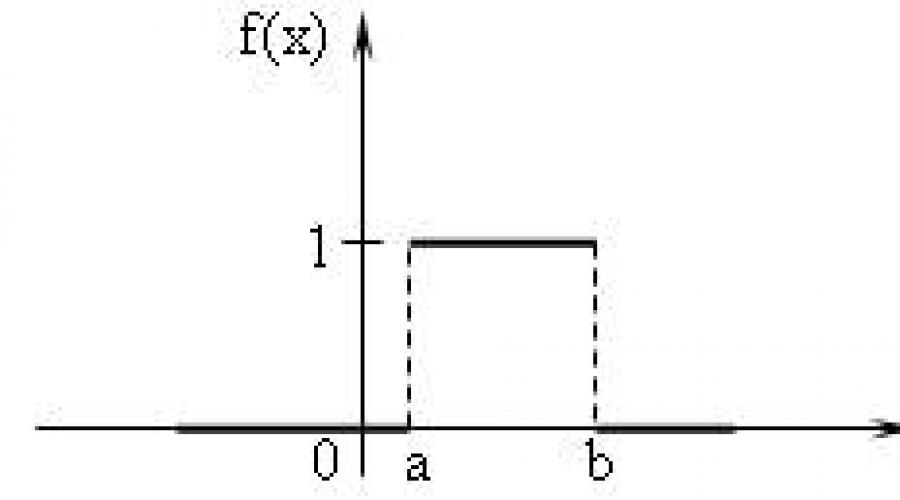
Uniform law is a symmetric distribution law of random variables (rectangle). The density of uniform distribution is given by the formula:
i.e., on the interval to which all possible values of the random variable belong, the density remains constant (Fig. 1).

Fig. 1 Probability density function and characteristics of uniform distribution
In simulation models of economic processes, uniform distribution is sometimes used to simulate simple (one-stage) work, when calculating according to network schedules of work, in military affairs - to simulate the timing of travel by subdivisions, the time of digging trenches and the construction of fortifications.
A uniform distribution is used if the only thing known about time intervals is that they have the maximum spread, and nothing is known about the probability distributions of these intervals.
1.3.2. Discrete distribution
Discrete distribution is represented by two laws:
1) binomial, where the probability of an event occurring in several independent tests is determined by the Bernoulli formula:
n - number of independent tests
m is the number of occurrences of an event in n tests.
2) the Poisson distribution, where, with a large number of tests, the probability of an event occurring is very small and is determined by the formula:
k is the number of occurrences of an event in several independent trials
Average number of occurrences of an event across multiple independent trials.
1.3.3. Normal distribution
The normal, or Gaussian, distribution is undoubtedly one of the most important and commonly used types of continuous distributions. It is symmetrical about the mathematical expectation.
Continuous random variable t has a normal probability distribution with parameters T and > Oh, if its probability density has the form (Fig. 2, Fig. 3):

where T- expected value M [t];
Fig. 2, Fig. 3 Probability density function and characteristics of the normal distribution
Any complex work on the objects of the economy consists of many short, sequential elementary components of work. Therefore, when estimating labor costs, it is always true that their duration is a random variable distributed according to the normal law.
In simulation models of economic processes, the law of normal distribution is used to model complex multi-stage work.
1.3.4. Exponential distribution
It also occupies a very important place in the systematic analysis of economic activity. Many phenomena obey this distribution law, for example:
1 time of receipt of the order for the enterprise;
2 customer visits to a supermarket;
3 telephone conversations;
4 the service life of parts and assemblies in a computer installed, for example, in accounting.
The exponential distribution function looks like this:
F (x) = at 0 Exponential distribution parameter,> 0. Exponential distributions are special cases of the gamma distribution. Rice. 5 Probability density function of gamma distribution In simulation models of economic processes, exponential distribution is used to model the intervals of incoming orders from multiple customers to a firm. In reliability theory, it is used to simulate the time interval between two successive faults. In communications and computer science - for modeling information flows. 1.3.5. Generalized Erlang Distribution P (t) = for t≥0; where K-elementary sequential components, distributed according to the exponential law. The generalized Erlang distribution is used to create both mathematical and simulation models. It is convenient to use this distribution instead of the normal distribution if the model is reduced to a purely mathematical problem. In addition, in real life there is an objective probability of the appearance of groups of applications as a reaction to some actions, therefore, group flows arise. The use of purely mathematical methods for studying the effects of such group flows in models is either impossible due to the lack of a way to obtain an analytical expression, or it is difficult, since analytical expressions contain a large systematic error due to numerous assumptions due to which the researcher was able to obtain these expressions. The generalized Erlang distribution can be used to describe one of the types of group flow. The emergence of group flows in complex economic systems leads to a sharp increase in the average duration of various delays (orders in queues, payment delays, etc.), as well as to an increase in the likelihood of risk events or insured events. 1.3.6. Triangular distribution Triangular distribution is more informative than uniform distribution. For this distribution, three quantities are determined - minimum, maximum and mode. The density function graph consists of two line segments, one of which increases with a change X from the minimum value to the mode, and the other decreases when changing X from mode value to maximum. The value of the mathematical expectation of a triangular distribution is equal to one third of the sum of the minimum, mode and maximum. The triangular distribution is used when the most probable value on a certain interval is known and the piecewise linear nature of the density function is assumed. Fig.5 Probability density function and characteristics of triangular distribution. The triangular distribution is easy to apply and interpret, but there must be a good reason for choosing it. In simulation models of economic processes, such a distribution is sometimes used to model the time of access to databases. 1.4. Planning a simulation computer experiment The simulation model, regardless of the chosen modeling system (for example, Pilgrim or GPSS), allows one to obtain the first two points and information about the distribution law of any quantity of interest to the experimenter (an experimenter is a subject who needs qualitative and quantitative conclusions about the characteristics of the process under study). 1.4.1. Cybernetic approach to the organization of experimental research of complex objects and processes. Experiment planning can be viewed as a cybernetic approach to organizing and conducting experimental research on complex objects and processes. The main idea of the method is the possibility of optimal control of an experiment under conditions of uncertainty, which is akin to the premises on which cybernetics is based. The purpose of most research works is to determine the optimal parameters of a complex system or the optimal conditions for the process: 1.determining the parameters of an investment project in conditions of uncertainty and risk; 2. the choice of structural and electrical parameters of the physical installation, providing the most advantageous mode of its operation; 3. obtaining the maximum possible reaction yield by varying the temperature, pressure and the ratio of reagents - in the tasks of chemistry; 4. selection of alloying components to obtain an alloy with the maximum value of any characteristic (toughness, tensile strength, etc.) - in metallurgy. When solving problems of this kind, it is necessary to take into account the influence of a large number of factors, some of which are not amenable to regulation and control, which extremely complicates a complete theoretical study of the problem. Therefore, they follow the path of establishing the basic laws through a series of experiments. The researcher was able to express the results of the experiment in a form convenient for their analysis and use through simple calculations. 1.4.2. Regression analysis and model experiment control Fig. 7 Example of averaging the experimental results Scatter of values η v in this case is determined not only by measurement errors, but mainly by the influence of interference z j... The complexity of the optimal control problem is characterized not only by the complexity of the dependence itself η v (v = 1, 2,…, n) but also the influence z j, which introduces an element of randomness into the experiment. Dependency graph η v (x i) determines the correlation between the quantities η v and x i, which can be obtained from the results of the experiment using the methods of mathematical statistics. Calculation of such dependencies for a large number of input parameters x i and significant influence of interference z j and is the main task of the researcher-experimenter. Moreover, the more difficult the task, the more effective the application of experimental planning methods becomes. There are two types of experiment: Passive; Active. At passive experiment the researcher only monitors the process (changes in its input and output parameters). Based on the results of the observations, a conclusion is made about the influence of the input parameters on the output. A passive experiment is usually performed on the basis of an ongoing economic or production process that does not allow active intervention by the experimenter. This method is not expensive, but it takes a lot of time. Active experiment is carried out mainly in laboratory conditions, where the experimenter has the ability to change the input characteristics according to a predetermined plan. Such an experiment leads to the goal faster. The corresponding approximation methods are called regression analysis. Regression analysis is a methodological toolkit for solving problems of forecasting, planning and analysis of economic activities of enterprises. The tasks of regression analysis are to establish the form of dependence between variables, to evaluate the regression function and to establish the influence of factors on the dependent variable, to estimate unknown values (forecast values) of the dependent variable. 1.4.3. Orthogonal planning of the second order. Orthogonal planning of the experiment (in comparison with non-orthogonal) reduces the number of experiments and greatly simplifies the calculations when obtaining the regression equation. However, such planning is feasible only if it is possible to conduct an active experiment. A practical tool for finding an extremum is a factorial experiment. The main advantages of the factorial experiment are simplicity and the possibility of finding an extreme point (with some error) if the unknown surface is sufficiently smooth and there are no local extrema. Two main disadvantages of the factorial experiment should be noted. The first one is that it is impossible to search for an extremum in the presence of stepwise discontinuities of an unknown surface and local extrema. The second - in the absence of means for describing the nature of the surface near the extreme point due to the use of the simplest linear regression equations, which affects the inertia of the control system, since in the control process it is necessary to carry out factorial experiments to select control actions. For control purposes, second-order orthogonal scheduling is most appropriate. An experiment usually consists of two stages. First, using a factorial experiment, an area is found where an extreme point exists. Then, in the region of existence of an extreme point, an experiment is carried out to obtain a regression equation of the 2nd order. The second-order regression equation allows you to immediately determine the control actions, without additional experiments or experiments. Additional experiment will be required only in cases where the response surface changes significantly under the influence of uncontrollable external factors (for example, a significant change in tax policy in the country will seriously affect the response surface reflecting the production costs of the enterprise 2. PRACTICAL WORK. In this section, we look at how the above theoretical knowledge can be applied to specific economic situations. The main objective of our coursework is to determine the effectiveness of an enterprise engaged in commercial activities For the implementation of the project, we have chosen the Pilgrim package. The Pilgrim package has a wide range of capabilities for simulating the temporal, spatial and financial dynamics of simulated objects. It can be used to create discrete-continuous models. The developed models have the property of collective management of the modeling process. Any blocks can be inserted into the model text using the standard C ++ language. The Pilgrim package is portable, i.e. porting to any other platform with a C ++ compiler. Models in the Pilgrim system are compiled and therefore have high performance, which is very important for working out management decisions and adaptive selection of options in a super-accelerated time scale. The object code obtained after compilation can be embedded into the developed software systems or transferred (sold) to the customer, since the tools of the Pilgrim package are not used when operating the models. The fifth version of Pilgrim is a software product created in 2000 on an object-oriented basis and taking into account the main positive properties of previous versions. The advantages of this system: Focus on joint modeling of material, informational and "monetary" processes; The presence of a developed CASE-shell, which allows constructing multilevel models in the mode of structural system analysis; Availability of interfaces with databases; The ability for the end user of the models to directly analyze the results thanks to the formalized technology for creating functional windows for observing the model using Visual C ++, Delphi or other means; The ability to control models directly in the process of their execution using special dialog boxes. Thus, the Pilgrim package is a good tool for creating both discrete and continuous models, has many advantages and greatly simplifies model creation. The object of observation is an enterprise that is engaged in the sale of the manufactured goods. For statistical analysis of the data on the functioning of the enterprise and comparison of the results obtained, all factors influencing the process of production and sale of goods were compared. The enterprise is engaged in the release of goods in small batches (the size of these batches is known). There is a market where these products are sold. The batch size of the purchased goods is generally a random variable. The structural diagram of the business process contains three layers. On two layers there are autonomous processes "Production" (Appendix A) and "Sales" (Appendix B), the schemes of which are independent from each other, since there are no ways to transfer transactions. The indirect interaction of these processes is carried out only through resources: material resources (in the form of finished products) and monetary resources (mainly through the current account). The management of cash resources takes place on a separate layer - in the process of "Cash transactions" (Appendix B). Let us introduce an objective function: the delay time of payments from the settlement account of Trs. Main control parameters: 1 unit price; 2 volume of the produced batch; 3 the amount of the loan requested from the bank. Fixing all other parameters: 4 batch release time; 5 the number of production lines; 6 interval of receipt of orders from buyers; 7 the range of sizes of the sold lot; 8 the cost of components and materials for the release of the batch; 9 starting capital on the current account; it is possible to minimize Trc for a specific market situation. The minimum Trc is achieved at one of the maximums of the average amount of money in the current account. Moreover, the probability of a risk event - non-payment of loan debts - is close to a minimum (this can be proved during a statistical experiment with the model). The first process " Production»(Appendix A) implements the basic elementary processes. Node 1 simulates the receipt of orders for the manufacture of batches of products from the company's management. Node 2 - an attempt to get a loan. An auxiliary transaction appears in this node - a request to the bank. Node 3 - waiting for a loan with this request. Node 4 is the administration of the bank: if the previous loan is returned, then a new one is provided (otherwise, the request is waiting in the queue). Node 5 transfers the loan to the company's current account. In node 6, the auxiliary request is destroyed, but the information that the loan has been provided is a “barrier” on the path of the next request for another loan (hold operation). The main transaction order passes through node 2 without delay. In node 7, payment for components is made if there is a sufficient amount on the current account (even if the loan has not been received). Otherwise, there is an expectation of either a loan or payment for the products sold. At node 8, a transaction is queued if all production lines are busy. Node 9 is manufacturing a batch of products. At node 10, an additional request for a loan repayment appears if the loan was previously allocated. This application goes to node 11, where money is transferred from the company's current account to the bank; if there is no money, then the application is awaiting. After the loan is repaid, this application is destroyed (in node 12); the bank has information that the loan has been repaid, and the company can issue the next loan (rels operation). The transaction order passes through node 10 without delay, and at node 13 it is destroyed. Further, it is considered that the batch is made and arrived at the finished product warehouse. The second process " Sales»(Appendix B) simulates the main functions for the sale of products. Node 14 is a generator of product buyer transactions. These transactions go to the warehouse (node 15), and if there is the requested quantity of goods, then the goods are released to the buyer; otherwise, buyer waits. Node 16 simulates goods issue and queue control. After receiving the goods, the buyer transfers the money to the company's current account (node 17). At node 18, the customer is considered served; the corresponding transaction is no longer needed and is destroyed. The third process “ Cash transactions»(Appendix B) simulates transactions in accounting. Posting requests come from the first layer from nodes 5, 7, 11 (process "Production") and from node 17 (process "Sales"). The dotted lines show the movement of funds on Account 51 ("Settlement account", node 20), account 60 ("Suppliers, contractors", node 22), account 62 ("Buyers, customers", node 21) and on account 90 (" Bank ", node 19). The conventional numbers roughly correspond to the chart of accounts of accounting. Node 23 mimics the work of a CFO. The processed transactions after accounting entries go back to the nodes where they came from; the numbers of these nodes are in the t → updown transaction parameter. The source code of the model is presented in Appendix D. This source code builds the model itself, i.e. creates all the nodes (represented in the structural diagram of the business process) and the links between them. The code can be generated by the Pilgrim (Gem) constructor, in which the processes are built in an object form (Appendix E). The model is created using Microsoft Developer Studio. Microsoft Developer Studio is a C ++ based application development package. After attaching additional libraries (Pilgrim.lib, comctl32.lib) and resource files (Pilgrim.res) to the project, we compile this model. After compilation, we get a ready-made model. A report file is automatically created, which stores the simulation results obtained after one run of the model. The report file is presented in Appendix D. 3. CONCLUSIONS ON THE BUSINESS MODEL "PRODUCTION EFFICIENCY" 1) Node number; 2) Node name; 3) Node type; 5) M (t) average waiting time; 6) Counter of inputs; 7) Remaining transactions; 8) The state of the node at this moment. The model consists of three independent processes: the main production process (Appendix A), the product sales process (Appendix B) and the cash flow management process (Appendix C). The main production process.
During the period of modeling the business process in node 1 ("Orders"), 10 applications for the manufacture of products were generated. The average order formation time is 74 days, as a result, one transaction was not included in the time frame of the modeling process. The remaining 9 transactions entered node 2 (“Fork1”), where the corresponding number of requests to the bank for a loan was created. The average waiting time is 19 days, which is the simulation time in which all transactions were satisfied. Further, it can be seen that 8 requests received a positive response in node 3 ("Issuance authorization"). The average time for obtaining a permit is 65 days. The load of this node averaged 70.4%. The state of the node at the end of the simulation time is closed, this is due to the fact that this node provides a new loan only if the previous one is returned, therefore, the loan at the end of the simulation has not been repaid (this can be seen from node 11). Node 5 transfers the loan to the company's current account. And, as can be seen from the table of results, the bank transferred 135,000 rubles to the company's account. At node 6, all 11 credit requests were destroyed. In node 7 ("Payments to suppliers"), payment for components was made in the amount of the entire loan received earlier (135,000 rubles). At node 8, we see that 9 transactions are queued. This happens when all production lines are busy. In node 9 ("Order fulfillment"), the direct production of products is carried out. It takes 74 days to make one batch of products. During the simulation period, 9 orders were completed. The load of this node was 40%. In node 13, orders for the manufacture of products were destroyed in the amount of 8 pieces. with the expectation that the batches are made and arrived at the warehouse. The average production time is 78 days. At node 10 (“Fork 2”), 0 additional applications for loan repayment were created. These applications were received at node 11 ("Return"), where a loan of 120,000 rubles was returned to the bank. After the loan was repaid, 7 applications for refund were destroyed in node 12. with an average time of 37 days. Product sales process.
Node 14 (Clients) generated 26 transactions-buyers of products with an average time of 28 days. One transaction is waiting in the queue. Then 25 transactions-buyers "turned" to the warehouse (node 15) for the goods. The warehouse utilization during the simulation period was 4.7%. Products from the warehouse were issued immediately - without delay. As a result of the issuance of products to customers, 1077 units remained in the warehouse. products, the receipt of the goods is not expected in the queue, therefore, upon receipt of the order, the enterprise can issue the required quantity of goods directly from the warehouse. Node 16 simulates the delivery of products to 25 customers (1 transaction in the queue). After receiving the goods, the customers paid for the received goods in the amount of 119160 rubles without delay. At node 18, all served transactions were destroyed. Cash flow management process.
In this process, we are dealing with the following accounting entries (requests for which come from nodes 5, 7, 11 and 17, respectively): 1 loan issued by the bank - 135,000 rubles; 2 payment to suppliers for components - 135,000 rubles; 3 bank loan repayment - 120,000 rubles; 4 funds from the sale of products - 119160 rubles were received on the current account. As a result of these postings, we received the following data on the distribution of funds across accounts: 1) Count. 90: Bank. 9 transactions were processed, one is waiting in the queue. The balance of funds is 9,970,000 rubles. Required - 0 rubles. 2) Count. 51: R / account. 17 transactions are served, one is waiting in the queue. The balance of funds is 14260 rubles. Required - 15,000 rubles. Consequently, when the simulation time is extended, the transaction in the queue cannot be serviced immediately due to the lack of funds on the company's account. 3) Count. 61: Customers. 25 transactions served. The balance of funds is 9,880,840 rubles. Required - 0 rubles. 4) Count. 60: Suppliers. 0 transactions serviced (the “Delivery of goods” process was not considered in this experiment). The balance of funds is 135,000 rubles. Required - 0 rubles. Node 23 mimics the work of a CFO. They served 50 transactions Analysis of the "Delay dynamics" graph.
As a result of running the model, in addition to the file containing tabular information, we get a graph of the dynamics of delays in the queue (Fig. 9). The graph of the dynamics of delays in the queue in the node "Calc. score 51 ”indicates that the delay increases over time. Delay of payments from the company's current account ≈ 18 days. This is a fairly high figure. As a result, the company makes payments less and less, and soon it is possible that the delay time exceeds the waiting time of the lender - this can lead to bankruptcy of the company. But, fortunately, these delays are not frequent, and therefore, this is a plus for this model. This situation can be resolved by minimizing the delay in payments for a specific market situation. The minimum delay time will be reached at one of the maximums of the average amount of money in the current account. In this case, the probability of non-payment of debts on loans will be close to a minimum. Evaluating the effectiveness of the model.
Based on the description of the processes, we can conclude that the processes of production and sales of products in general work effectively. The main problem of the model is the cash flow management process. The main problem of this process is debts to repay a bank loan, thereby causing a shortage of funds in the current account, which will not allow free manipulation of the funds received, because they need to be directed to repay the loan. As we learned from the analysis of the "Delay dynamics" graph, in the future the company will be able to repay accounts payable on time, but not always in clearly indicated lines Therefore, we can conclude that at the moment the model is quite effective, but requires the smallest improvements. The generalization of the results of statistical processing of information was carried out by analyzing the results of the experiment. The graph of delays in the "Settlement account" node shows that, throughout the entire simulation period, the delays in the node are mostly at the same level, although delays appear occasionally. It follows that the increase in the likelihood of a situation where an enterprise may be on the verge of bankruptcy is extremely low. Therefore, the model is quite acceptable, but, as mentioned above, it requires minor improvements. CONCLUSION Systems that are complex in terms of internal connections and large in terms of the number of elements are economically difficult to direct methods of modeling and often, for construction and study, they switch to simulation methods. The emergence of the latest information technologies increases not only the capabilities of modeling systems, but also allows the use of a wider variety of models and methods of their implementation. The improvement of computing and telecommunications technology has led to the development of computer modeling methods, without which it is impossible to study processes and phenomena, as well as the construction of large and complex systems. Based on the work done, we can say that the importance of modeling in the economy is very great. Therefore, a modern economist should be well versed in economic and mathematical methods, be able to practically apply them to simulate real economic situations. This makes it possible to better assimilate the theoretical issues of the modern economy, contributes to the improvement of the level of qualifications and the general professional culture of a specialist. With the help of various business models, it is possible to describe economic objects, patterns, connections and processes not only at the level of an individual firm, but also at the state level. And this is a very important fact for any country: it is possible to predict ups and downs, crises and stagnation in the economy. BIBLIOGRAPHY 1. Emelyanov A.A., Vlasova E.A. Computer modeling - M .: Moscow state. University of Economics, Statistics and Informatics, 2002. 2. Locks OO, Tolstopyatenko AV, Cheremnykh Yu.N. Mathematical Methods in Economics, M., Business and Service, 2001. 3. Kolemaev VA, Mathematical Economics, M., UNITI, 1998. 4. Naylor T. Machine simulation experiments with models of economic systems. - M .: Mir, 1975 .-- 392 p. 5. Councils B.Ya., Yakovlev S.A. System modeling. - M .: Higher. Shk., 2001. 6. Shannon R.E. Simulation of systems: science and art. - M .: Mir, 1978. 7.www.thrusta.narod.ru APPENDIX A Business model diagram "Enterprise efficiency" APPENDIX B The process of selling products of the business model "Enterprise Efficiency" APPENDIX B The cash flow management process of the Enterprise Efficiency business model APPENDIX D Model source code APPENDIX E Model Report File APPENDIX E Students, graduate students, young scientists who use the knowledge base in their studies and work will be very grateful to you. University of International Business. On the topic: Simulation modeling in economics Completed by student gr. Economy Tazhibaev Ermek Almaty 2009 Plan Introduction 1. Definition of the concept of "simulation" 2. Simulation of reproduction processes in the oil and gas industry 3. Monte Carlo method as a kind of simulation 4. Example. Assessment of geological reserves Conclusion Introduction Both analytical and statistical models are widely used in operations research. Each of these types has advantages and disadvantages. Analytical models are coarser, take into account fewer factors, and always require some kind of assumptions and simplifications. On the other hand, the calculation results for them are easier to see, more clearly reflect the main regularities inherent in the phenomenon. And, most importantly, analytical models are more suited to finding optimal solutions. Statistical models, in comparison with analytical ones, are more accurate and detailed, do not require such rough assumptions, allow taking into account a large (in theory - an infinitely large) number of factors. But they also have their drawbacks: cumbersomeness, poor visibility, high consumption of computer time, and most importantly, the extreme difficulty of finding optimal solutions that have to be looked for "by touch" by guesswork and trial. The best work in operations research is based on the combined use of analytical and statistical models. The analytical model makes it possible to understand the phenomenon in general terms, to outline, as it were, the outline of the basic laws. Any refinements can be obtained using statistical models. Simulation is applied to processes in which human will can interfere from time to time. The person in charge of the operation can, depending on the current situation, make certain decisions, just as a chess player, looking at the board, chooses his next move. Then a mathematical model is set in motion, which shows how the situation is expected to change in response to this decision and what consequences it will lead to after some time. The next "current decision" is made taking into account the real new situation, and so on. As a result of repeated repetition of such a procedure, the manager, as it were, "gains experience", learns from his own and others' mistakes and gradually learns to make the right decisions - if not optimal, then almost optimal. 1.
Definition of "simulation modeling" In modern literature, there is no single point of view on what is meant by imitation modeling. So there are different interpretations: In the first, a simulation model is understood as a mathematical model in the classical sense; In the second, this term is retained only for those models in which random influences are played out (imitated) in one way or another; In the third, it is assumed that the simulation model differs from the usual mathematical one in a more detailed description, but the criterion by which one can say when the mathematical model ends and the simulation begins is not introduced; Simulation is applied to processes in which human will can interfere from time to time. The person in charge of the operation can, depending on the current situation, make certain decisions, just like a chess player looking at the board chooses his next move. Then a mathematical model is set in motion, which shows how the situation is expected to change in response to this decision and what consequences it will lead to after some time. The next current decision is made taking into account the real new situation, etc. As a result of repeated repetition of this procedure, the manager seems to "gain experience", learns from his own and others' mistakes and gradually learn to make the right decisions - if not optimal, then almost optimal. Let's try to illustrate the simulation process by comparing it with a classical mathematical model. Stages of the process of building a mathematical model of a complex system: 1. The main questions about the behavior of the system are formulated, the answers to which we want to get with the help of the model. 2. From the set of laws governing the behavior of the system, those are selected whose influence is significant in the search for answers to the questions posed. 3. In addition to these laws, if necessary, for the system as a whole or its individual parts, certain hypotheses about the functioning are formulated. Practice serves as the criterion for the adequacy of the model. Difficulties in building a mathematical model of a complex system: If the model contains many links between elements, various nonlinear constraints, a large number of parameters, etc. Real systems are often subject to the influence of random various factors, the accounting of which analytically presents very great difficulties, often insurmountable with a large number of them; The possibility of comparing the model and the original with this approach is available only at the beginning. These difficulties determine the use of simulation modeling. It is implemented in the following stages: 1. As before, the main questions about the behavior of a complex system are formulated, the answers to which we want to receive. 2. The system is decomposed into simpler parts-blocks. 3. Laws and "plausible" hypotheses regarding the behavior of both the system as a whole and its individual parts are formulated. 4. Depending on the questions posed to the researcher, the so-called system time is introduced, which simulates the course of time in a real system. 5. The necessary phenomenological properties of the system and its individual parts are specified in a formalized way. 6. The random parameters appearing in the model are compared with some of their implementations, which remain constant for one or more system time cycles. Next, new implementations are found. 2.
Simulation of reproduction processes in the oil and gas industry The current stage of development of the oil and gas industry is characterized by the increasing complexity of relations and interaction of natural, economic, organizational, environmental and other factors of production both at the level of individual enterprises and oil and gas producing regions, and at the industry-wide level. In the oil and gas industry, production is distinguished by long periods, the separation of the production and technological process in time (prospecting and exploration, development and construction, oil, gas and condensate production), the presence of lag shifts and delays, the dynamism of the resources used and other factors, the values of many of which are probabilistic nature. The values of these factors change systematically due to the commissioning of new fields, as well as the lack of confirmation of the expected results for those in development. This forces the enterprises of the oil and gas industry to periodically revise plans for the reproduction of fixed assets and redistribute resources in order to optimize the results of production and economic activities. When drawing up plans, significant assistance to persons preparing a draft economic decision can be provided by the use of methods of mathematical modeling, including simulation. The essence of these methods lies in the repeated reproduction of variants of planning decisions with subsequent analysis and selection of the most rational of them according to the established system of criteria. Using a simulation model, you can create a single structural diagram that integrates functional controls (strategic, tactical and operational planning) for the main production processes of the industry (prospecting, exploration, development, production, transportation, oil and gas processing). 3.
Monte Carlo method as a varietysimulation The date of birth of the Monte Carlo method is considered to be 1949, when an article titled "The Monte Carlo method" appeared. American mathematicians J. Neumann and S. Ulam are considered the creators of this method. In the USSR, the first articles on the Monte Carlo method were published in 1955-1956. It is curious that the theoretical basis of the method has been known for a long time. Moreover, some statistical problems were sometimes calculated using random samples, that is, in fact, by the Monte Carlo method. However, before the advent of electronic computers (computers), this method could not find any widespread use, because modeling random variables "manually is a very laborious work. Thus, the emergence of the Monte Carlo method as a very universal numerical method became possible only thanks to the appearance COMPUTER. The very name “Monte Carlo” comes from the city of Monte Carlo in the Principality of Monaco, famous for its gambling house. The idea of the method is extremely simple and it consists in the following. Instead of describing the process with the help of an analytical apparatus (differential or algebraic equations), a "drawing" of a random phenomenon is performed using a specially organized procedure that includes randomness and gives a random result. In reality, the concrete realization of a random process develops differently each time; similarly, as a result of statistical modeling, each time we get a new, different from the others implementation of the process under study. What can she give us? Nothing in itself, just like, say, one case of a patient cured with the help of some kind of medicine. It is another matter if there are many such implementations. This set of realizations can be used as some kind of artificially obtained statistical material that can be processed by the usual methods of mathematical statistics. After such processing, any characteristics of interest to us can be obtained: probabilities of events, mathematical expectations and variances of random variables, etc. When simulating random phenomena by the Monte Carlo method, we use randomness itself as a research apparatus, make it work for us. This is often easier than trying to build an analytical model. For complex operations in which a large number of elements (machines, people, organizations, auxiliary means) are involved, in which random factors are complexly intertwined, where the process is clearly not Markovian, the statistical modeling method, as a rule, turns out to be simpler than analytical (and often the only possible). In essence, any probabilistic problem can be solved by the Monte Carlo method, but it becomes justified only when the drawing procedure is simpler, and not more complicated than analytical calculation. Let's give an example when the Monte Carlo method is possible, but extremely unreasonable. Suppose, for example, three independent shots are fired at some target, each of which hits the target with a probability of 1/2. It is required to find the probability of at least one hit. An elementary calculation gives us the probability of at least one hit equal to 1 - (1/2) 3 = 7/8. The same problem can be solved by "drawing", statistical modeling. Instead of “three shots” we will throw “three coins”, counting, say, the coat of arms for a hit, and tails for a “miss”. The experiment is considered "successful" if at least one of the coins has a coat of arms. Let's make a lot of experiments, calculate the total number of "successes" and divide by the number N of experiments performed. Thus, we get the frequency of the event, and it is close to the probability for a large number of experiments. Well, what then? Such a technique could only be applied by a person who does not know the theory of probability at all, nevertheless, in principle, it is possible. The Monte Carlo method is a numerical method for solving mathematical problems by simulating random variables. Let's consider a simple example illustrating the method. Example 1. Suppose we need to calculate the area of a flat figure S. It can be an arbitrary figure with a curved border, defined graphically or analytically, connected or consisting of several pieces. Let it be the figure shown in fig. 1, and assume that it is all located within the unit square. Choose N random points inside the square. Let F denote the number of points that fall inside S. It is geometrically obvious that the area of S is approximately equal to the ratio F / N. The larger N, the greater the accuracy of this estimate. Two features of the Monte Carlo method. The first feature of the method is the simple structure of the computational algorithm. The second feature of the method is the calculation error, as a rule, proportional to D / N2, where D is some constant, N is the number of tests. This shows that in order to reduce the error by a factor of 10 (in other words, to get one more correct decimal point in the answer), you need to increase N (that is, the amount of work) by a factor of 100. It is clear that it is impossible to achieve high accuracy in this way. Therefore, it is usually said that the Monte Carlo method is especially effective in solving those problems in which the result is needed with a small accuracy (5-10%). The way to use the Monte Carlo method is, in theory, quite simple. To obtain an artificial random sample from a set of quantities described by a certain probability distribution function, one should: 1. Construct a graph or table of the cumulative distribution function based on a series of numbers reflecting the process under study (and not on the basis of a series of random numbers), and the values of the random process variable are plotted along the abscissa axis (x), and the probability values (from 0 to 1) - along the ordinate (y). 2.Using a random number generator, select a random decimal number in the range from 0 to 1 (with the required number of digits). 3. Draw a horizontal line from the point on the ordinate corresponding to the selected random number, to the intersection with the probability distribution curve. 4. From this intersection point the perpendicular to the abscissa axis. b. Repeat steps 2-5 for all required random variables, following the order in which they were written. The general meaning is easy to understand with a simple example: the number of calls to the telephone exchange within 1 minute corresponds to the following distribution: Number of calls Probability Cumulative probability O 0.10 0.10 Suppose we want to conduct a thought experiment for five time periods. Let's build a graph of the cumulative probability distribution. Using the random number generator, we get five numbers, each of which is used to determine the number of calls in a given time interval. Time period Random number Number of calls Taking a few more such samples, we can make sure that if the numbers used are really evenly distributed, then each of the values of the investigated quantity will appear with the same frequency as in the unreal world ", and we will get the results typical for the behavior of the system under investigation. Let's go back to the example. To calculate, we had to select random points in a unit square. How to do it physically? Let's imagine such an experiment. Fig. 1. (on a larger scale) with an S and a square hung on the wall as a target. The shooter, who was at some distance from the wall, shoots N times, aiming at the center of the square. Of course, all the bullets will not land exactly in the center: they will hit N random points on the target. Is it possible to estimate the area S. It is clear that with a high qualification of the shooter, the result of the experiment will be very poor, since almost all the bullets will fall near the center and hit S. It is easy to understand that our method of calculating the area will be valid only when the random points are not just “random”, but also “evenly scattered” over the whole square. In operations research problems, the Monte Carlo method is used in three main roles: 1) when modeling complex, complex operations, where there are many interacting random factors; 2) when checking the applicability of simpler, analytical methods and clarifying the conditions for their applicability; 3) in order to develop amendments to analytical formulas such as "empirical formulas" in technology. 4.
Example... Assessment of geological reserves To assess the amount of recoverable reserves, it is necessary, first of all, to determine the amount of total or geological reserves. Analysis of structural traps. To assess the content of oil and / or gas in a structural trap, exploration and production geologists and geophysicists must study the nature of the structural trap. Such a study is necessary to determine the possible value of the geological reserves. The area of changes in reserves is determined by a combination of the following estimated indicators: volume of sedimentary rocks (RV), porosity (F), first water saturation (Sw), effective thickness (NP) g. Determination of the likely values of the parameter. At this stage, geologists must evaluate the significance of the probabilities for the parameters used in calculating the reserves. Interval values of probabilities are assigned to each parameter, based on expert assessments of geologists Analysis of probability graphs. Accumulated probability graphs. The continuous curve represents the probability that the value of the parameter in question will be "equal to or greater" than the value at that point on the horizontal axis that is crossed by the vertical line projected from the curve, perpendicular to the vertical axis for any value from 0 to 100%. The curve is based on histogram data, which are shown as shaded bars. Histograms represent expert judgment by prospecting and field geologists and geophysicists who provide information in the following form: In our opinion, the probability that the volume of the reservoir is in the range from 0 to 390 kft is 10%; We estimate the probability that the volume of rocks is between 380 and 550 cubic meters. feet is 15% and so on. These geologists' estimates are accumulated, and the result is a generalized probability curve. Based on this curve, it is possible to extrapolate the values of the expected probabilities for the studied parameters. Calculation of geological reserves. The volume of geological reserves is calculated using the following formula: RVxFx (l-Sw) x NPx -, where Fv is the coefficient of bringing oil to surface conditions. Using averages to get a rough estimate of the geological reserves. When evaluating the approximate amount of oil in the field, we will use the following parameter values: Average rock volume is 1.35 million acre-feet (1 acre-foot = 7760 barrels or about 1230 m3) Average porosity - 17% Average water saturation - 20% Average effective power - 75% The reduction factor is 1.02 (there is no free gas in reservoir conditions). Now let's substitute these values into the formula (1.35 x 10) x (17%) x (1 - 20%) x (75%) x (i.e.: 1350000x0.17x0.8x0.75x0.98) = 134,946 acre feet or 134946x7760 = 1047413760, i.e. approximately 1.047 billion barrels of oil (165 million m3, 141 million tons). The more common way is the Monte Carlo method. First of all, it is necessary to build histograms and cumulative probability curves for each parameter. For each of these curves, it is necessary to randomly select a point corresponding to a probability from 0 to 100%. After that, you need to substitute the value of the parameter corresponding to this probability into the equation. Then you can calculate the geological reserves at these values of the parameters and calculate the total probability For example: For a 50% cumulative probability, we have a 25% probability that the volume of the rocks will be 690,000 acre-feet. For a 20% cumulative probability, we have a 35% probability that the porosity will be 21%. For a 25% cumulative probability, we have a 25% probability that the water content is 33% The 80% cumulative probability indicates a 32% probability that the effective power will be 74%. The coefficient of bringing oil to surface conditions is taken equal to 1.02. Using these values, we calculate the geological reserves: (0.69 x 1 0) x (2 1%) x (l - 33%) x (74%) x ---- Having decided, we get approximately: 521 million barrels of oil (82 million m3, 70 million tons). The result of this calculation is significantly less than when using the average values of the parameters. We need to know the probability of this outcome. To determine the probability that in-place reserves will amount to 521 million barrels of oil, we calculate the total probability: 0.25 x 0.35 x 0.20 x 0.35 x 1.0 = 0.006125, i.e. the probability is 0.6125% - not very good! This procedure is repeated many times, for which we used a computer program. This gives us a reasonable probability distribution of the geological reserves. As a result of the implementation of the program, the volume of geological oil reserves was predicted: it is most likely that the volume of oil will be 84658 acre-feet, or about 88.5 million tons. Using the cumulative probability distribution. In the next step, using the graph, it is necessary to select several estimates along with their probabilities. For each of these values, the following are calculated: production dynamics, development project options. These calculations can then be used to estimate the capital operating costs for each inventory value selected from the schedule. Economic indicators are then analyzed for each inventory value. After some time, and after a certain number of wells have been drilled, the success rate is calculated using the formula. Success rate = number of wells given oil \ number of drills. wells The probability of success is plotted over a period of several years. For example, for a notional area, the success rate is plotted after nine years of operation. Conditional lines are drawn through the corresponding success values, then an envelope curve is drawn through their centers. The extreme points of these lines correspond to the maximum level of success, and the central curve corresponds to the most probable level of success. The values of the probabilities are determined on the basis of the subjective judgments of the field geologists. The level of reserves per well is determined in a similar way. Using the success rate and average reserves per well, the probability of reaching a certain level of reserves necessary for drawing up a drilling program and determining the number of required wells is estimated. Conclusion The main disadvantage of analytical models is that they inevitably require some kind of assumptions, in particular, about the "Markov character" of the process. The acceptability of these assumptions can not always be assessed without control calculations, but they are made by the Monte Carlo method. Figuratively speaking, the Monte Carlo method plays the role of a kind of OTK in operations research problems. Statistical models do not require major assumptions and simplifications. In principle, anything “climbs” into the statistical model - any distribution laws, any complexity of the system, the multiplicity of its states. The main disadvantage of statistical models is their cumbersomeness and laboriousness. The huge number of implementations required to find the desired parameters with acceptable accuracy requires a lot of computer time. In addition, the results of statistical modeling are much more difficult to comprehend than calculations based on analytical models, and, accordingly, it is more difficult to optimize the solution (you have to "grope" blindly). The right mix of analytical and statistical methods in operations research is a matter of art, instinct, and experience of the researcher. Often, using analytical methods, it is possible to describe some "subsystems" allocated in a large system, and then from such models as from "bricks", build a building of a large, complex model. Bibliography 1. Wentzel E.S. "Operations Research", Moscow "Soviet Radio" 1972 2. Sobol I.M. "Monte Carlo method", Moscow "Science", 1985 3. "Economic and mathematical methods and applied models", ed. Fedoseeva V.V., Moscow "Unity" 2001 The concept of simulation modeling, its application in economics. Stages of the process of constructing a mathematical model of a complex system, criteria for its adequacy. Discrete Event Modeling. The Monte Carlo method is a type of simulation. test, added 12/23/2013 Statistical model of a stochastic process. Numerical Monte Carlo method. Types of imitation, its advantages and possibilities. A simple simulation model of a document processing system. Using Siman for modeling. Its main modeling blocks. presentation added on 10/22/2014 Calculation of the economic effect of the bank. Simulation based on pre-defined dependencies. Exponential distribution function. Adjustment of customer service time at cash desks and queue advancement. test, added 10/03/2008 Calculation of the economic effect of the bank. Algorithm for simulation of the checkout hall operation. Exponential distribution function. Adjustment of customer service time at cash desks and queue advancement. Listing of the program. test, added 10/03/2008 Simulation modeling as a method for analyzing economic systems. Pre-project survey of a printing services company. Investigation of a given system using a model of the "Markov process" type. Calculation of the service time for one request. term paper, added 10/23/2010 Capital investment efficiency. Statistical methods for assessing the feasibility of investments with risk. Sensitivity analysis, scenarios. Establishment of nominal and limit values of uncertain factors. Simulation modeling of Monte Carlo. test, added 10/27/2008 The concept of a uniformly distributed random variable. Multiplicative congruent method. Simulation of continuous random variables and discrete distributions. Algorithm for simulation of economic relations between a lender and a borrower. term paper, added 01/03/2011 Review of methods for solving the problem. Calculation of the number of customers, revenue, average queue size and number of refusals during the simulation period. Process modeling algorithm, development of its software implementation. Machine experiment with the developed model. term paper, added 01/15/2011 Description of computer modeling. Advantages, stages and approaches to building simulation modeling. The content of the basic concept of structuring the GPSS modeling language. Plan Evaluation and Review Method (PERT). Simulation in the GPSS system. term paper added 03/03/2011 The method of simulation in the development of economic and mathematical models to account for the uncertainty of enterprise statistics. Functioning of a simulation model for manufacturing a small-sized chair: operating time and equipment load factors. Simulation modeling is a method that allows you to build models that describe processes as they would in reality. Such a model can be “played” in time for both one test and a given set of them. In this case, the results will be determined by the random nature of the processes. Based on these data, one can obtain fairly stable statistics. The relevance of this topic lies in the fact that simulation modeling on digital computers is one of the most powerful research tools, in particular, of complex dynamic systems. Like any computer simulation, it makes it possible to carry out computational experiments with systems that are still being designed and to study systems that are not expedient for full-scale experiments with which, due to safety or high cost considerations. At the same time, due to its proximity in form to physical modeling, this research method is available to a wider range of users. Simulation modeling is a research method in which the system under study is replaced by a model that describes the real system with sufficient accuracy and experiments are carried out with it in order to obtain information about this system. The goals of such experiments can be very different - from identifying the properties and patterns of the system under study, to solving specific practical problems. With the development of computer technology and software, the range of application of simulation in the field of economics has expanded significantly. At present, it is used both for solving problems of intra-firm management and for modeling management at the macroeconomic level. Let's consider the main advantages of using simulation modeling in the process of solving financial analysis problems. In the process of simulation, the researcher deals with four main elements: Real system; Logical and mathematical model of the simulated object; Simulation (machine) model; The computer on which the imitation is carried out is a directed computational experiment. To describe the dynamics of the simulated processes in imitation modeling, a mechanism for setting the model time is implemented. These mechanisms are built into the control programs of any simulation system. If the behavior of one component of the system were simulated on a computer, then the execution of actions in the simulation model could be carried out sequentially, by recalculating the time coordinate. To ensure the simulation of parallel events in a real system, a certain global variable (providing synchronization of all events in the system) t0 is introduced, which is called the model (or system) time. There are two main ways to change t0: Incremental (fixed change intervals apply model time); Event-by-event (variable intervals are applied model time, while the step size is measured by the interval until the next event). In the case of the stepwise method, the time advance occurs with the smallest possible constant step length (principle t). These algorithms are not very efficient in terms of using computer time to implement them. By-event method (the principle of “special states”). In it, the time coordinates change only when the state of the system changes. In event-by-event methods, the length of the time shift step is maximum possible. The model time from the current moment changes to the nearest moment of the next event occurrence. The use of the event-by-event method is preferable if the frequency of occurrence of events is low, then a large step length will speed up the course of the model time. When solving many problems of financial analysis, models are used that contain random variables, the behavior of which cannot be controlled by decision-makers. Such models are called stochastic. The use of simulation allows conclusions to be drawn about possible outcomes based on the probability distributions of random factors (quantities). Stochastic simulation is often referred to as the Monte Carlo method. From all of the above, we can conclude that simulation allows you to take into account the maximum possible number of environmental factors to support management decisions and is the most powerful tool for analyzing investment risks. The need for its application in domestic financial practice is due to the peculiarities of the Russian market, which is characterized by subjectivity, dependence on non-economic factors and a high degree of uncertainty. The simulation results can be supplemented by probabilistic and statistical analysis and, in general, provide the manager with the most complete information about the degree of influence of key factors on the expected results and possible scenarios for the development of events. The process becomes a method that allows you to construct patterns that describe processes in such a way as if they actually functioned. By applying them, it is possible to obtain stable and reliable statistics. Based on these data, you can choose the optimal path for the development of the organization. The simulation method is a research method in which a specific system will be replaced by one that has sufficient accuracy in describing the real one. Experiments must be carried out with it in order to obtain reliable information. Such a procedure will allow you to comprehend the essence of the phenomenon, without resorting in this case to real changes in the object until the required time. Simulation of business processes is a special case of mathematical modeling. The fact is that there is a class of objects for which analytical models have not been developed for various reasons. Or, for them, there is no system of methods for applying an innovative solution. In such cases, simulation of economic processes is used. It is used when: Simulation processes have several types. Let's consider them in more detail. Agent modeling is an innovative area that is widely used to explore decentralized systems. The dynamics of their functioning is determined not so much by global laws and rules, but, on the contrary, these principles are the result of the individual activities of the members of this group. Therefore, in this case, the purpose and objectives of the models are to get ideas about these fundamental principles, the behavior of the selected system. But it will be necessary to proceed from assumptions about the individual, private behavior of its individual objects, as well as their relationships in systems. An agent becomes a special entity that has activity and autonomy in behavior, is able to make and apply decisions in accordance with a set of specific rules, interact with the existing environment, and also independently change itself. Discrete-event modeling is a modeling approach that offers to abstract from the existing events, considering a number of basic events in the system. We are talking about "waiting", "processing orders", "moving with the load", "unloading" and so on. Such modeling is very well developed and has a huge scope of application - from logistics, as well as service systems to manufacturing and transport systems. In general, the method is ideal for any situation; was founded by J. Gordon in the middle of the twentieth century. System dynamics is an imitation modeling of economic processes, when graphs, diagrams, calculations will be built for the object under study, reflecting the causal relationships and global influences of some criteria on others in a certain period of time. Further, the system created on their basis is simulated on a computer. Thanks to this, there is a real opportunity to understand the essence of what is happening, and to identify the existing connections of cause and effect between phenomena and objects. System dynamics helps to build models for the development of cities, business processes, production systems, environmental development, population, epidemics, and so on. Course project On the subject: "Modeling of production and economic processes" On the topic: "Simulation of economic processes" Introduction I. Basic concepts of the theory of modeling economic systems and processes 1 Concept of modeling 1.2 Model concept II. Basic concepts of the theory of modeling economic systems and processes 2.1 Improvement and development of economic systems 2 Components of a simulation model III. Simulation Basics 3.1 Simulation model and its features 2 The essence of simulation IV. Practical part 1 Problem statement 2 Solving the problem Conclusion List of used literature Application Introduction Simulation modeling, linear programming and regression analysis in terms of range and frequency of use have long occupied the first three places among all methods of operations research in economics. In imitation modeling, the algorithm that implements the model reproduces the process of the system's functioning in time and space, and the elementary phenomena constituting the process are simulated while preserving its logical temporal structure. At present, modeling has become a fairly effective means of solving complex problems of automation of research, experiments, and design. But to master modeling as a working tool, its wide capabilities and to develop the modeling methodology further is possible only with full mastery of the techniques and technology of practical solution of problems of modeling the processes of functioning of systems on a computer. This goal is pursued by this workshop, which focuses on the methods, principles and main stages of modeling within the framework of the general modeling methodology, as well as discusses the issues of modeling specific system options and instills the skills of using modeling technology in the practical implementation of models of the functioning of systems. The problems of queuing systems on which simulation models of economic, information, technological, technical and other systems are based are considered. Methods of probabilistic modeling of discrete and random continuous variables are presented, which allow taking into account random influences on the system when modeling economic systems. The demands made by modern society for a specialist in the field of economics are steadily growing. Currently, successful activity in almost all spheres of the economy is not possible without modeling the behavior and dynamics of the development of processes, studying the features of the development of economic objects, considering their functioning in various conditions. Software and hardware should be the first assistants here. Instead of learning from your mistakes or from the mistakes of other people, it is advisable to consolidate and check the knowledge of reality with the results obtained on computer models. Simulation modeling is the most illustrative, it is used in practice for computer modeling of options for resolving situations in order to obtain the most effective solutions to problems. Simulation modeling allows the study of the analyzed or projected system according to the operational study scheme, which contains interrelated stages: · Development of a conceptual model; · Development and software implementation of a simulation model; · Checking the correctness, reliability of the model and assessing the accuracy of the simulation results; · Planning and conducting experiments; · making decisions. This makes it possible to use simulation modeling as a universal approach for decision-making under conditions of uncertainty, taking into account the factors that are difficult to formalize in the models, and also to apply the basic principles of the systems approach to solving practical problems. The widespread implementation of this method in practice is hindered by the need to create software implementations of simulation models that recreate the dynamics of the modeled system functioning in model time. Unlike traditional programming methods, the development of a simulation model requires a restructuring of the principles of thinking. It is not for nothing that the principles underlying simulation modeling gave impetus to the development of object programming. Therefore, the efforts of developers of software tools for simulation are aimed at simplifying software implementations of simulation models: for these purposes, specialized languages and systems are created. Simulation software has changed in its development over several generations, from modeling languages and automation tools for constructing models to program generators, interactive and intelligent systems, and distributed modeling systems. The main purpose of all these tools is to reduce the complexity of creating software implementations of simulation models and experiment with models. One of the first modeling languages to make it easier to write simulations was GPSS, an end product by Geoffrey Gordon at IBM in 1962. Currently, there are translators for DOS operating systems - GPSS / PC, for OS / 2 and DOS - GPSS / H and for Windows - GPSS World. Learning this language and creating models allows you to understand the principles of developing simulation programs and learn how to work with simulation models. (General Purpose Simulation System) - a modeling language that is used to build event-driven discrete simulation models and conduct experiments using a personal computer. GPSS is a language and translator. Like every language, it contains a vocabulary and grammar with which models of a particular type of system can be developed. I. Basic concepts of the theory of modeling economic systems and processes 1.1 Concept of modeling Modeling refers to the process of building, learning, and applying models. It is closely related to such categories as abstraction, analogy, hypothesis, etc. The modeling process necessarily includes the construction of abstractions, and inferences by analogy, and the construction of scientific hypotheses. The main feature of modeling is that it is a method of indirect cognition using substitute objects. The model acts as a kind of cognitive tool that the researcher puts between himself and the object, and with the help of which he studies the object of interest. Any socio-economic system is a complex system in which tens and hundreds of economic, technical and social processes interact, constantly changing under the influence of external conditions, including scientific and technological progress. In such conditions, the management of socio-economic and production systems turns into a complex task that requires special tools and methods. Modeling is one of the main methods of cognition, it is a form of reflection of reality and consists in clarifying or reproducing certain properties of real objects, objects and phenomena with the help of other objects, processes, phenomena, or with the help of an abstract description in the form of an image, plan, map , a set of equations, algorithms and programs. In the most general sense, a model is understood as a logical (verbal) or mathematical description of components and functions that reflect the essential properties of a modeled object or process, usually considered as systems or system elements from a certain point of view. The model is used as a conditional image, designed to simplify the study of the object. In principle, not only mathematical (sign), but also material models are applicable in economics, but material models have only demonstrative value. There are two points of view on the essence of modeling: This is the study of objects of knowledge on models; This is the construction and study of models of real-life objects and phenomena, as well as supposed (constructed) objects. The modeling capabilities, that is, the transfer of the results obtained during the construction and study of the model, to the original are based on the fact that the model in a certain sense reflects (reproduces, simulates, describes, imitates) some features of the object of interest to the researcher. Modeling as a form of reflection of reality is widespread, and a sufficiently complete classification of possible types of modeling is extremely difficult, if only due to the ambiguity of the concept of "model", which is widely used not only in science and technology, but also in art and in everyday life. The word "model" comes from the Latin word "modulus", meaning "measure", "sample". Its original meaning was associated with the art of building, and in almost all European languages it was used to denote an image or prototype, or a thing, similar in some respect to another thing. Among socio-economic systems, it is advisable to single out the production system (PS), which, unlike systems of other classes, contains a consciously acting person performing the functions of management (decision-making and control) as the most important element. In accordance with this, various divisions of enterprises, the enterprises themselves, research and design organizations, associations, industries and, in some cases, the national economy as a whole, can be considered as PS. The nature of the similarity between the modeled object and the model is different: Physical - the object and the model have the same or similar physical nature; Structural - there is a similarity between the structure of the object and the structure of the model; functional - the object and the model perform similar functions under the appropriate action; Dynamic - there is a correspondence between the sequentially changing states of the object and the model; Probabilistic - there is a correspondence between processes of a probabilistic nature in the object and the model; Geometric - there is a correspondence between the spatial characteristics of the object and the model. Modeling is one of the most common ways to study processes and phenomena. Modeling is based on the principle of analogy and allows you to study an object under certain conditions and taking into account the inevitable one-sided point of view. An object that is difficult to study is not studied directly, but through consideration of another, similar to it and more accessible - the model. By the properties of the model, it usually turns out to be possible to judge the properties of the object under study. But not all properties, but only those that are similar both in the model and in the object, and at the same time are important for research. Such properties are called essential. Is there a need for mathematical modeling of the economy? In order to be convinced of this, it is enough to answer the question: is it possible to carry out a technical project without having an action plan, that is, drawings? The same situation takes place in the economy. Do you need to prove the need to use economic and mathematical models for making managerial decisions in the field of economics? Under these conditions, the economic and mathematical model turns out to be the main means of experimental research of the economy, since it has the following properties: Simulates a real economic process (or behavior of an object); Has a relatively low cost; Can be reused; Takes into account various conditions for the functioning of the object. The model can and should reflect the internal structure of an economic object from given (definite) points of view, and if it is unknown, then only its behavior, using the “Black box” principle. In principle, any model can be formulated in three ways: As a result of direct observation and study of the phenomena of reality (phenomenological method); Extraction from a more general model (deductive method); Generalizations of more particular models (inductive method, that is, a proof by induction). Models, endless in their variety, can be classified according to a wide variety of criteria. First of all, all models can be subdivided into physical and descriptive ones. We constantly deal with both those and others. In particular, descriptive models include models in which the modeled object is described using words, drawings, mathematical dependencies, etc. These models include literature, art, music. In the management of economic processes, economic and mathematical models are widely used. There is no established definition of an economic and mathematical model in the literature. Let's take the following definition as a basis. An economic and mathematical model is a mathematical description of an economic process or an object, carried out for the purpose of researching or managing them: a mathematical record of the economic problem being solved (therefore, the terms problem and model are often used as synonyms). Models can also be classified according to other criteria: Models describing the momentary state of the economy are called static. Models that show the development of the simulation object are called dynamic. Models that can be built not only in the form of formulas (analytical representation), but also in the form of numerical examples (numerical representation), in the form of tables (matrix representation), in the form of a special kind of graphs (network representation). 2 Model concept At the present time, it is impossible to name an area of human activity in which dressing methods would not be used to one degree or another. Meanwhile, there is no generally accepted definition of the concept of a model. In our opinion, the following definition deserves preference: a model is an object of any nature, which is created by a researcher in order to obtain new knowledge about the original object and reflects only the essential (from the developer's point of view) properties of the original. Analyzing the content of this definition, the following conclusions can be drawn: ) any model is subjective, it bears the stamp of the individuality of the researcher; ) any model is homomorphic, i.e. it reflects not all, but only the essential properties of the original object; ) it is possible that there are many models of the same original object, differing in the objectives of the study and the degree of adequacy. A model is considered adequate to the original object if it reflects the laws of the process of functioning of a real system in the external environment with a sufficient degree of approximation at the level of understanding of the modeled process by the researcher. Mathematical models can be divided into analytical, algorithmic (simulation) and combined. Analytical modeling is characterized by the fact that systems of algebraic, differential, integral or finite-difference equations are used to describe the processes of system functioning. The analytical model can be investigated by the following methods: a) analytical, when they strive to obtain in general form explicit dependencies for the desired characteristics; b) numerical, when, not being able to solve equations in general form, they strive to obtain numerical results for specific initial data; c) qualitative, when, without having an explicit solution, it is possible to find some properties of the solution (for example, to estimate the stability of the solution). In algorithmic (imitation) modeling, the process of the system functioning in time is described, and the elementary phenomena that make up the process are simulated, while maintaining their logical structure and sequence of flow in time. Simulation models can also be deterministic and statistical. The general goal of modeling in the decision-making process was formulated earlier - this is the determination (calculation) of the values of the selected performance indicator for various strategies of the operation (or options for implementing the designed system). When developing a specific model, the purpose of the simulation should be refined taking into account the efficiency criterion used. Thus, the goal of modeling is determined both by the goal of the operation being investigated and by the planned way of using the research results. For example, a problem situation requiring a decision is formulated as follows: to find an option for building a computer network that would have the minimum cost while meeting the performance and reliability requirements. In this case, the purpose of modeling is to find the network parameters that provide the minimum value of the PE, in the role of which is the cost. The problem can be formulated differently: choose the most reliable one from several options of the computer network configuration. Here, one of the reliability indicators (mean time between failures, probability of failure-free operation, etc.) is selected as a PE, and the purpose of modeling is a comparative assessment of network options for this indicator. The above examples allow us to remind that the choice of the performance indicator itself does not yet determine the “architecture” of the future model, since at this stage its concept has not been formulated, or, as they say, the conceptual model of the system under study has not been defined. II. Basic concepts of the theory of modeling economic systems and processes 2.1 Improvement and development of economic systems Simulation is the most powerful and versatile method of research and evaluation of the efficiency of systems, the behavior of which depends on the influence of random factors. Such systems include an aircraft, a population of animals, and an enterprise operating in conditions of poorly regulated market relations. The simulation is based on a statistical experiment (Monte Carlo method), the implementation of which is practically impossible without the use of computer technology. Therefore, any simulation model is ultimately a more or less complex software product. Of course, like any other program, the simulation model can be developed in any general-purpose programming language, even in Assembly language. However, in this case, the following problems arise on the path of the developer: Knowledge is required not only of the subject area to which the studied system belongs, but also of the programming language, and at a sufficiently high level; The development of specific procedures for ensuring a statistical experiment (generation of random influences, planning an experiment, processing the results) can take no less time and effort than the development of the system's model itself. And finally, one more, perhaps the most important problem. In many practical problems, interest is not only (and not so much) a quantitative assessment of the efficiency of a system, but rather its behavior in a given situation. For such an observation, the researcher must have appropriate "viewing windows", which could be closed if necessary, moved to another place, changed the scale and form of the observed characteristics, etc., without waiting for the end of the current model experiment. The simulation model in this case acts as a source of the answer to the question: "what will happen if ...". Implementing such capabilities in a universal programming language is not easy. Currently, there are quite a few software products that allow you to simulate processes. These packages include: Pilgrim, GPSS, Simplex and a number of others. At the same time, at the present time on the Russian market of computer technologies there is a product that makes it possible to very effectively solve these problems - the MATLAB package, which contains the Simulink visual modeling tool. Simulink is a tool that allows you to quickly model a system and get indicators of the expected effect and compare them with the effort required to achieve them. There are many different types of models: physical, analog, intuitive, etc. A special place among them is occupied by mathematical models, which, according to Academician A.A. Samarsky, "are the greatest achievement of the scientific and technological revolution of the XX century." Mathematical models are divided into two groups: analytical and algorithmic (which are sometimes called imitation). At present, it is impossible to name an area of human activity in which modeling methods would not be used to one degree or another. Economic activity is no exception. However, in the field of simulation modeling of economic processes, some difficulties are still observed. In our opinion, this circumstance is explained by the following reasons. Economic processes occur largely spontaneously, uncontrollably. They do not lend themselves well to attempts at volitional control on the part of political, state and economic leaders of individual industries and the country's economy as a whole. For this reason, economic systems are difficult to study and formalized description. Specialists in the field of economics, as a rule, have insufficient mathematical training in general and in mathematical modeling in particular. Most of them do not know how to formally describe (formalize) the observed economic processes. This, in turn, does not allow us to establish whether this or that mathematical model is adequate for the economic system under consideration. Specialists in the field of mathematical modeling, not having at their disposal a formalized description of the economic process, cannot create a mathematical model adequate to it. The existing mathematical models, which are commonly called models of economic systems, can be conditionally divided into three groups. The first group includes models that fairly accurately reflect any one side of a certain economic process taking place in a relatively small-scale system. From the point of view of mathematics, they represent very simple relationships between two or three variables. Usually these are algebraic equations of the 2nd or 3rd degree, in the extreme case, a system of algebraic equations that requires the use of the iteration method (successive approximations) to solve. They find application in practice, but are not of interest from the point of view of specialists in the field of mathematical modeling. The second group includes models that describe real processes occurring in small and medium-sized economic systems that are exposed to random and uncertain factors. The development of such models requires making assumptions to resolve the uncertainties. For example, you need to specify the distributions of random variables related to the input variables. To a certain extent, this artificial operation raises doubts about the reliability of the simulation results. However, there is no other way to create a mathematical model. Among the models of this group, the most widespread are the models of the so-called queuing systems. There are two flavors of these models: analytical and algorithmic. Analytical models do not take into account the effect of random factors and therefore can only be used as first approximation models. With the help of algorithmic models, the process under study can be described with any degree of accuracy at the level of its understanding by the task manager. The third group includes models of large and very large (macroeconomic) systems: large trade and industrial enterprises and associations, branches of the national economy and the country's economy as a whole. The creation of a mathematical model of an economic system of this scale is a complex scientific problem, the solution of which is within the power of only a large research institution. 2.2 Components of the simulation model Numerical modeling deals with three kinds of values: raw data, calculated variable values, and parameter values. Arrays with these values occupy separate areas on an Excel sheet. The initial real data, samples or series of numbers, are obtained by direct field observation or in experiments. Within the framework of the modeling procedure, they remain unchanged (it is clear that, if necessary, the sets of values can be supplemented or reduced) and play a double role. Some of them (independent environment variables, X) serve as the basis for calculating model variables; most often these are characteristics of natural factors (the course of time, photoperiod, temperatures, abundance of feed, dose of toxicant, volumes of pollutants discharge, etc.). Another part of the data (dependent variables of the object, Y) is a quantitative characteristic of the state, reactions or behavior of the object of research, which was obtained under certain conditions, under the action of registered environmental factors. In a biological sense, the first group of meanings does not depend on the second; on the contrary, object variables depend on environment variables. Data is entered into an Excel sheet from the keyboard or from a file in the usual mode of working with a spreadsheet. The model calculated data reproduce the theoretically conceivable state of the object, which is determined by the previous state, the level of the observed environmental factors and is characterized by the key parameters of the process under study. In the ordinary case, when calculating model values (Y M i) for each time step (i), parameters (A), the characteristic of the previous state (Y M i -1) and the current levels of environmental factors (X i) are used: Y M i = f (A, Y M i-1, X i, i), where () is the accepted form of the ratio of parameters and variables of the environment, the type of model, = 1, 2,… T or i = 1, 2,… n. Calculations of the characteristics of the system using model formulas for each time step (for each state) make it possible to form an array of model explicit variables (Y М), which should exactly repeat the structure of the array of real dependent variables (Y), which is necessary for the subsequent adjustment of model parameters. Formulas for calculating model variables are entered into the cells of an Excel worksheet manually (see the section Useful tricks). Model parameters (A) make up the third group of values. All parameters can be represented as a set: = (a 1, a 2,…, a j,…, a m), where j is the parameter number, m is the total number of parameters, and place it in a separate block. It is clear that the number of parameters is determined by the structure of the accepted model formulas. Occupying a separate position on the Excel sheet, they play the most significant role in modeling. The parameters are designed to characterize the very essence, the mechanism of the observed phenomena. The parameters must have a biological (physical) meaning. For some tasks, it is necessary that the parameters calculated for different data sets can be compared. This means that they sometimes have to be accompanied by their own statistical errors. The relationships between the components of the simulation system form a functional unity focused on achieving a common goal - the assessment of model parameters (Fig. 2.6, Table 2.10). In the implementation of individual functions indicated by arrows, several elements are simultaneously involved. In order not to clutter up the picture, the graphical presentation and randomization blocks are not reflected in the diagram. The simulation system is designed to service any changes in the model's structures, which, if necessary, can be made by the researcher. Basic constructions of simulation systems, as well as possible ways of their decomposition and integration are presented in the section Frames of simulation systems. simulation economic series III. Simulation Basics 1 Simulation model and its features Simulation modeling is a kind of analog modeling, implemented using a set of mathematical tools, special simulating computer programs and programming technologies that allow, through analogous processes, to conduct a targeted study of the structure and functions of a real complex process in the computer memory in the "simulation" mode, to optimize some of it parameters. The simulation model is an economic and mathematical model, the study of which is carried out by experimental methods. The experiment consists in observing the results of calculations for various specified values of the introduced exogenous variables. The simulation model is a dynamic model due to the fact that it contains such a parameter as time. A simulation model is also called a special software package that allows you to simulate the activity of any complex object. The emergence of simulation has been associated with a "new wave" in economics-thematic modeling. The problems of economic science and practice in the field of management and economic education, on the one hand, and the growth of computer productivity, on the other, have caused the desire to expand the scope of "classical" economic and mathematical methods. There was some disappointment in the possibilities of normative, balance, optimization and game-theoretic models, which at first deservedly attracted by the fact that they bring an atmosphere of logical clarity and objectivity to many problems of economic management, and also lead to a "reasonable" (balanced, optimal, compromise) solution ... It was not always possible to fully comprehend the a priori goals and, moreover, to formalize the criterion of optimality and (or) restrictions on feasible solutions. Therefore, many attempts to apply such methods nevertheless began to lead to unacceptable, for example, unrealizable (albeit optimal) solutions. Overcoming the difficulties that arose went along the path of refusal from full formalization (as is done in normative models) of the procedures for making socio-economic decisions. The preference was given to a reasonable synthesis of the intellectual capabilities of an expert and the information power of a computer, which is usually implemented in dialogue systems. One trend in this direction is the transition to “semi-normative” multi-criteria human-machine models, the second is the shift of the center of gravity from prescriptive models oriented towards the “conditions - decision” scheme to descriptive models that answer the question “what will happen if .. . ". Simulation modeling is usually resorted to in cases where the dependencies between the elements of the simulated systems are so complex and indefinite that they cannot be formally described in the language of modern mathematics, i.e., using analytical models. Thus, researchers of complex systems are forced to use simulation modeling when purely analytical methods are either inapplicable or unacceptable (due to the complexity of the corresponding models). In imitation modeling, the dynamic processes of the original system are replaced by the processes simulated by the modeling algorithm in the abstract model, but observing the same ratios of durations, logical and temporal sequences, as in the real system. Therefore, the simulation method could be called algorithmic or operational. By the way, such a name would be more apt, since imitation (translated from Latin - imitation) is the reproduction of something by artificial means, that is, modeling. In this regard, the currently widely used name "simulation modeling" is tautological. In the process of imitating the functioning of the system under study, as in an experiment with the original itself, certain events and states are recorded, according to which the necessary characteristics of the quality of the functioning of the system under study are then calculated. For systems, for example, information and computing services, as such dynamic characteristics can be defined: The performance of data processing devices; Service queue length; Waiting time for service in queues; The number of requests that left the system without service. In imitation modeling, processes of any degree of complexity can be reproduced if there is a description of them, given in any form: formulas, tables, graphs, or even verbally. The main feature of simulation models is that the process under study is, as it were, "copied" on a computer, therefore simulation models, in contrast to analytical models, allow: To take into account in the models a huge number of factors without gross simplifications and assumptions (and, consequently, to increase the adequacy of the model to the system under study); It is enough to simply take into account the uncertainty factor caused by the random nature of many model variables in the model; All this allows us to make a natural conclusion that simulation models can be created for a wider class of objects and processes. 2 The essence of simulation The essence of simulation is in purposeful experimentation with the simulation model by "playing" on it various options for the functioning of the system with their respective economic analysis. It should be noted right away that the results of such experiments and the corresponding economic analysis should be formalized in the form of tables, graphs, nomograms, etc., which greatly simplifies the decision-making process based on the simulation results. Having listed above a number of advantages of simulation models and simulation, we also note their disadvantages, which must be remembered in the practical use of simulation. It: Lack of well-structured principles for constructing simulation models, which requires a significant study of each specific case of its construction; Methodological difficulties in finding optimal solutions; Increased requirements for the speed of computers on which simulation models are implemented; Difficulties in collecting and preparing representative statistics; The uniqueness of simulation models, which does not allow the use of ready-made software products; The complexity of the analysis and understanding of the results obtained as a result of a computational experiment; Quite a large expenditure of time and money, especially when searching for optimal trajectories of the behavior of the system under study. The number and essence of the listed shortcomings is very impressive. However, given the great scientific interest in these methods and their extremely intensive development in recent years, we can confidently assume that many of the above disadvantages of simulation modeling can be eliminated both in conceptual and applied terms. Simulation of a controlled process or a controlled object is a high-level information technology that provides two types of actions performed by a computer: ) work on the creation or modification of the simulation model; ) operation of the simulation model and interpretation of the results. Simulation of economic processes is usually used in two cases: To manage a complex business process, when the simulation model of a controlled economic object is used as a tool% in the loop of an adaptive control system created on the basis of information technologies; When conducting experiments with discrete-continuous models of complex economic objects to obtain and track their dynamics in emergency situations associated with risks, the full-scale modeling of which is undesirable or impossible. The following typical tasks can be distinguished, which are solved by means of simulation modeling in the management of economic objects: Modeling logistics processes to determine time and cost parameters; Management of the implementation process of an investment project at various stages of its life cycle, taking into account possible risks and tactics of allocating funds; Analysis of clearing processes in the operation of a network of credit institutions (including application to offsetting processes in the Russian banking system); Forecasting the financial results of the enterprise for a specific period of time (with an analysis of the dynamics of the balance on the accounts); Business reengineering of an insolvent enterprise (changing the structure and resources of a bankrupt enterprise, after which, using a simulation model, you can make a forecast of the main financial results and give recommendations on the advisability of one or another option for reconstruction, investment or lending to production activities); A simulation system that provides the creation of models for solving the listed tasks must have the following properties: The possibility of using simulation programs in conjunction with special economic and mathematical models and methods based on control theory; Instrumental methods of structural analysis of a complex economic process; The ability to model material, monetary and information processes and flows within a single model, in general, model time; The possibility of introducing a mode of constant refinement when obtaining output data (basic financial indicators, temporal and spatial characteristics, risk parameters, etc.) and conducting an extreme experiment. Many economic systems are essentially queuing systems (QS), that is, systems in which, on the one hand, there are requirements for the performance of any services, and on the other hand, these requirements are satisfied. IV. Practical part 1 Problem statement Investigate the dynamics of an economic indicator based on the analysis of a one-dimensional time series. For nine consecutive weeks, the demand Y (t) (mln rubles) for credit resources of a financial company was recorded. The time series Y (t) of this indicator is given in the table. Required: Check for abnormal observations. Build a linear model Y (t) = a 0 + a 1 t, the parameters of which are estimated by the least squares (Y (t)) - calculated, modeled values of the time series). Assess the adequacy of the constructed models using the properties of independence of the residual component, randomness and compliance with the normal distribution law (when using the R / S criterion, take the tabulated boundaries 2.7-3.7). Estimate the accuracy of the models based on the use of the average relative error of approximation. Using the two constructed models, forecast the demand for the next two weeks (the confidence interval of the forecast is calculated with the confidence probability p = 70%) The actual values of the indicator, the results of modeling and forecasting are presented graphically. 4.2 Solving the problem 1). The presence of anomalous observations leads to distortion of the simulation results, therefore it is necessary to make sure that there are no anomalous data. To do this, we will use Irwin's method and find the characteristic number () (Table 4.1). ; The calculated values are compared with the tabular values of the Irwin test, and if they turn out to be more than the tabular values, then the corresponding value of the series level is considered anomalous. Appendix 1 (Table 4.1) All the obtained values were compared with the table values, they do not exceed them, that is, there are no anomalous observations. ) Build a linear model, the parameters of which are estimated by the OLS (- calculated, modeled values of the time series). To do this, we will use Data Analysis in Excel. Appendix 1 ((Figure 4.2) Figure 4.1) The result of the regression analysis is contained in the table Appendix 1 (table 4.2 and 4.3.) In the second column of the table. 4.3 contains the coefficients of the regression equation a 0, a 1, the third column contains the standard errors of the coefficients of the regression equation, and the fourth column contains t statistics used to test the significance of the coefficients of the regression equation. The regression equation for the dependence of (demand for credit resources) on (time) has the form Appendix 1 (fig. 4.5) 3) Assess the adequacy of the constructed models. 1. Let's check independence (absence of autocorrelation) using d - Darbin - Watson criterion according to the formula: Appendix 1 (Table 4.4) Because the calculated value of d falls within the range from 0 to d 1, i.e. in the range from 0 to 1.08, then the independence property is not satisfied, the levels of a number of residuals contain autocorrelation. Consequently, the model for this criterion is inadequate. 2. We will check the randomness of the levels of a number of residuals on the basis of the turning point criterion. P> The number of pivot points is 6. Appendix 1 (Figure 4.5) The inequality holds (6> 2). Consequently, the property of randomness is satisfied. The model is adequate for this criterion. 3. The correspondence of a number of residuals to the normal distribution law is determined using the RS - criterion: The maximum level of a number of residues, The minimum level of a number of residues, Standard deviation, The calculated value falls within the interval (2.7-3.7), therefore, the property of normal distribution is fulfilled. The model is adequate for this criterion. 4. Checking that the mathematical expectation of the levels of a number of residuals is equal to zero. In our case, therefore, the hypothesis about the equality of the mathematical expectation of the values of the residual series to zero is fulfilled. Table 4.3 summarizes the analysis data for a number of residues. Appendix 1 (Table 4.6) 4) Estimate the accuracy of the model based on the use of the average relative error of approximation. To assess the accuracy of the resulting model, we will use the indicator of the relative approximation error, which is calculated by the formula: Calculation of the relative error of approximation Appendix 1 (Table 4.7) If the error calculated by the formula does not exceed 15%, the model's accuracy is considered acceptable. 5) According to the constructed model, forecast the demand for the next two weeks (the confidence interval of the forecast is calculated with the confidence probability p = 70%). Let's use the Excel function STYUDRESIST. Appendix 1 (Table 4.8) To build an interval forecast, we calculate the confidence interval. We take the value of the significance level, therefore, the confidence level is 70%, and the Student's test at The width of the confidence interval is calculated by the formula: We calculate the upper and lower boundaries of the forecast (Table 4.11). Appendix 1 (Table 4.9) 6) The actual values of the indicator, the results of modeling and forecasting are presented graphically. Let's transform the selection schedule, adding it with the forecast data. Appendix 1 (Table 4.10) Conclusion An economic model is defined as a system of interrelated economic phenomena expressed in quantitative characteristics and presented in a system of equations, i.e. is a system of formalized mathematical description. For the purposeful study of economic phenomena and processes and the formulation of economic conclusions - both theoretical and practical, it is advisable to use the method of mathematical modeling. Particular interest is shown in methods and means of simulation modeling, which is associated with the improvement of information technologies used in simulation systems: the development of graphical shells for constructing models and interpreting the output results of modeling, the use of multimedia tools, Internet solutions, etc. In economic analysis, simulation is the most versatile tool in the field of financial, strategic planning, business planning, production management and design. Mathematical modeling of economic systems The most important property of mathematical modeling is its versatility. This method allows, at the design and development stages of an economic system, to form various variants of its model, to carry out repeated experiments with the obtained model variants in order to determine (based on the specified criteria for the functioning of the system) the parameters of the system being created, necessary to ensure its efficiency and reliability. In this case, the acquisition or production of any equipment or hardware is not required to perform the next calculation: you just need to change the numerical values of the parameters, initial conditions and modes of operation of the complex economic systems under study. Methodologically, mathematical modeling includes three main types: analytical, simulation and combined (analytical and simulation) modeling. An analytical solution, if possible, gives a more complete and visual picture that allows you to obtain the dependence of the simulation results on the set of initial data. In this situation, you should move on to using simulation models. The simulation model, in principle, allows you to reproduce the entire process of the functioning of the economic system while maintaining the logical structure, connections between phenomena and their sequence in time. Simulation modeling allows you to take into account a large number of real details of the functioning of a modeled object and is indispensable at the final stages of creating a system, when all strategic issues have already been resolved. It can be noted that simulation is intended for solving problems of calculating system characteristics. The number of options to be evaluated should be relatively small, since the implementation of simulation modeling for each option for building an economic system requires significant computing resources. The fact is that a fundamental feature of simulation is the fact that statistical methods must be used to obtain meaningful results. This approach requires multiple repetitions of the simulated process with varying values of random factors, followed by statistical averaging (processing) of the results of individual single calculations. The use of statistical methods, which is inevitable in simulation, requires a lot of computer time and computational resources. Another drawback of the simulation method is the fact that to create sufficiently meaningful models of the economic system (and at those stages of creating an economic system when simulation modeling is used, very detailed and meaningful models are needed), significant conceptual and programming efforts are required. Combined modeling allows you to combine the advantages of analytical and simulation modeling. To improve the reliability of the results, a combined approach based on a combination of analytical and simulation modeling methods should be used. In this case, analytical methods should be applied at the stages of property analysis and synthesis of the optimal system. Thus, from our point of view, a system of comprehensive training of students in the means and methods of both analytical and simulation modeling is needed. Organization of practical training Students learn ways to solve optimization problems, which are reduced to linear programming problems. The choice of this modeling method is due to the simplicity and clarity of both the meaningful formulation of the corresponding problems and the methods of their solution. In the process of performing laboratory work, students solve the following typical tasks: transport problem; the task of distributing the resources of the enterprise; the problem of equipment placement, etc. 2) Studying the basics of simulation of production and non-production queuing systems in the environment of GPSS World (General Purpose System Simulation World). The methodological and practical issues of creating and using simulation models in the analysis and design of complex economic systems and decision-making in the implementation of commercial and marketing activities are considered. Methods of description and formalization of simulated systems, stages and technology of construction and use of simulation models, issues of organizing purposeful experimental research on simulation models are studied. List of used literature The main 1. Akulich I.L. Mathematical programming in examples and problems. - M .: Higher school, 1986 2. Vlasov M. P., Shimko P. D. Modeling of economic processes. - Rostov-on-Don, Phoenix - 2005 (electronic textbook) 3. Yavorskiy V.V., Amirov A.Zh. Economic informatics and information systems (laboratory workshop) - Astana, Folio, 2008 4. Simonovich S.V. Computer Science, Peter, 2003 5. Vorobiev N.N. Game theory for economists - cybernetics. - M .: Science, 1985 (electronic textbook) 6. Alesinskaya T.V. Economic and mathematical methods and models. - Tagan Rog, 2002 (electronic textbook) 7. Gershhorn A.S. Mathematical programming and its application in economic calculations. -M. Economics, 1968 Additionally 1. Darbinyan M.M. Trade stocks and their optimization. - M. Economics, 1978 2. Johnston D.J. Economic methods. - M .: Finance and Statistics, 1960 3. Epishin Yu.G. Economic and mathematical methods and planning of consumer cooperation. - M .: Economics, 1975 4. Zhitnikov S.A., Birzhanova Z.N., Ashirbekova B.M. Economic and mathematical methods and models: Textbook. - Karaganda, publishing house KEU, 1998 5. Locks OO, Tolstopyatenko AV, Cheremnykh Yu.N. Mathematical methods in economics. - M .: DIS, 1997 6. Ivanilov Yu.P., Lotov A.V. Mathematical methods in economics. - M .: Science, 1979 7. Kalinina V.N., Pankin A.V. Math statistics. M .: 1998 8. Kolemaev V.A. Mathematical economics. M., 1998 9. Kremer N.Sh., Putko B.A., Trishin I.M., Fridman M.N. Operation research in economics. Study guide - M .: Banks and stock exchanges, UNITI, 1997 10. Spirin A.A :, Fomin G.P. Economic and mathematical methods and models in trade. - M .: Economics, 1998 Annex 1 Table 4.1
Table 4.2
Odds Standard error t-statistics Y-intersection a 0 Table 4.3 Withdrawing residues
WITHDRAWAL REMAINING Observation Predicted Y Table 4.6
Checked property Used statistics Name meaning Independence d-test inadequate Accident Pivot point criterion adequate Normality RS test adequate Average = 0? Student's t-statistic adequate Conclusion: the statistics model is inadequate Table 4.7
Predicted Y Table 4.9 Forecast table 
Figure 4 shows the characteristics of the gamma distribution, as well as a graph of its density function for various values of these characteristics.  This is an asymmetrical distribution. It occupies an intermediate position between exponential and normal. The probability density of the Erlang distribution is represented by the formula:
Figure 5 shows the characteristics of a triangular distribution and a graph of its probability density function.
If we consider the dependence of one of the characteristics of the system η v (x i) as a function of only one variable x i(Fig. 7), then at fixed values x i we will get different values η v (x i)
. 
Rice
.8
Boot
the form
Microsoft Developer Studio

Fig.9 Delay graph in the "Settlement account" node.
Send your good work in the knowledge base is simple. Use the form below
Similar documents

 ,
, ![]() .
.
![]() ,
,
![]()
 ,
, ![]()
![]()
![]() , where
, where ![]()
![]() is equal to 1.12.
is equal to 1.12. , where
![]() (found from table 4.1)
(found from table 4.1)

