The general scheme of the study of the function online. Full function exploration and plotting

Today we invite you to explore and graph the function with us. After carefully studying this article, you will not have to sweat for a long time to complete this kind of task. Exploring and plotting a function is not easy, the work is voluminous, requiring maximum attention and accuracy of calculations. To facilitate the perception of the material, we will study the same function step by step, explain all our actions and calculations. Welcome to the amazing and exciting world of mathematics! Go!

Domain

In order to explore and plot a function, you need to know several definitions. Function is one of the basic (basic) concepts in mathematics. It reflects the relationship between several variables (two, three or more) with changes. The function also shows the dependence of the sets.

Imagine that we have two variables that have a certain range of variation. So, y is a function of x, provided that each value of the second variable corresponds to one value of the second. In this case, the variable y is dependent, and it is called a function. It is customary to say that the variables x and y are in. For greater clarity of this dependence, a function graph is plotted. What is a function graph? This is a set of points on the coordinate plane, where each value of x corresponds to one value of y. Graphs can be different - straight line, hyperbola, parabola, sinusoid and so on.

It is impossible to plot a function graph without research. Today we will learn how to conduct research and plot a function graph. It is very important to make notes during the research. This will make the task much easier. The most convenient research plan:

1. Domain.
2. Continuity.
3. Even or odd parity.
4. Periodicity.
5. Asymptotes.
6. Zeros.
7. Constancy of signs.
8. Increasing and decreasing.
9. Extremes.
10. Convexity and concavity.

Let's start with the first point. Let's find the domain of definition, that is, on what intervals our function exists: y = 1/3 (x ^ 3-14x ^ 2 + 49x-36). In our case, the function exists for any values ​​of x, that is, the domain is equal to R. It can be written as follows xÎR.

Continuity

Now we are going to investigate the break function. In mathematics, the term "continuity" appeared as a result of the study of the laws of motion. What is infinite? Space, time, some dependencies (an example is the dependence of the variables S and t in motion problems), the temperature of the heated object (water, frying pan, thermometer, and so on), a continuous line (that is, one that can be drawn without tearing it off the sheet pencil).

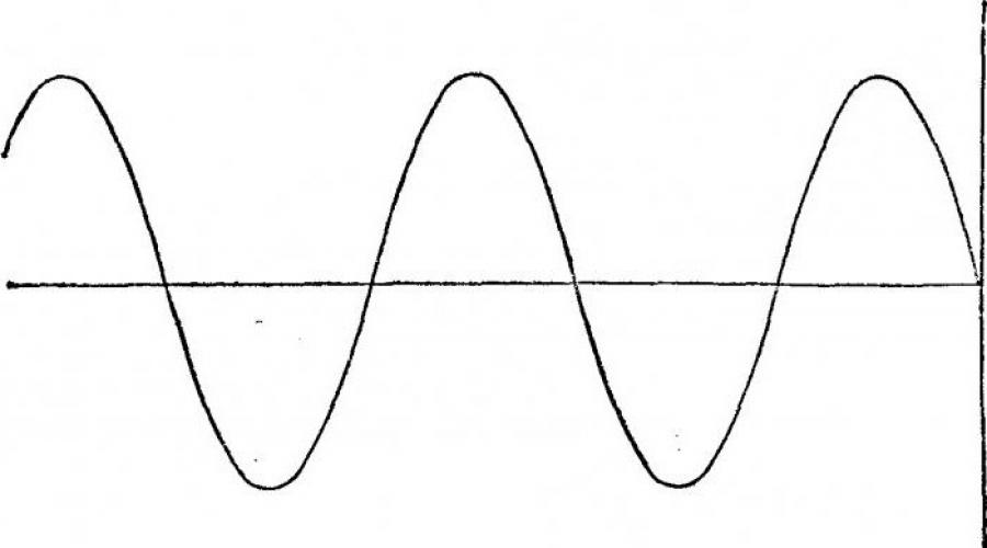
A chart is considered to be continuous if it does not break at some point. One of the clearest examples of such a graph is a sine wave, which you can see in the picture in this section. The function is continuous at some point x0 if a number of conditions are met:

• a function is defined at this point;
• the right and left limits at the point are equal;
• the limit is equal to the value of the function at the point x0.

If at least one condition is not met, the function is said to be broken. And the points at which the function is discontinuous are usually called discontinuity points. An example of a function that will "break" when displayed graphically is: y = (x + 4) / (x-3). Moreover, y does not exist at the point x = 3 (since it is impossible to divide by zero).

In the function that we are examining (y = 1/3 (x ^ 3-14x ^ 2 + 49x-36)), everything turned out to be simple, since the graph will be continuous.

Even, odd

Now examine the function for parity. First, a little theory. An even function is one that satisfies the condition f (-x) = f (x) for any value of the variable x (from the range of values). Examples include:

• module x (the graph looks like a daw, the bisector of the first and second quarters of the graph);
• x squared (parabola);
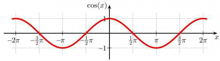
• cosine x (cosine).

Note that all of these plots are symmetrical when viewed in relation to the ordinate (i.e. y).

What, then, is called an odd function? These are those functions that satisfy the condition: f (-x) = - f (x) for any value of the variable x. Examples:

• hyperbola;
• cubic parabola;
• sinusoid;
• tangentoid and so on.

Please note that these functions are symmetrical about the point (0: 0), that is, the origin. Based on what has been said in this section of the article, an even and an odd function must have the property: x belongs to the set of definitions and -x too.

Let us examine the function for parity. We can see that it doesn't fit any of the descriptions. Therefore, our function is neither even nor odd.

Asymptotes

Let's start with the definition. An asymptote is a curve that is as close to the graph as possible, that is, the distance from a point tends to zero. In total, there are three types of asymptotes:

• vertical, that is, parallel to the y-axis;
• horizontal, that is, parallel to the x axis;
• inclined.

As for the first type, data straight lines should be looked for at some points:

• break;
• ends of the domain of definition.

In our case, the function is continuous, and the domain is equal to R. Therefore, there are no vertical asymptotes.

The graph of a function has a horizontal asymptote, which meets the following requirement: if x tends to infinity or minus infinity, and the limit is equal to a certain number (for example, a). In this case, y = a - this is the horizontal asymptote. In the function we are investigating, there are no horizontal asymptotes.

The oblique asymptote only exists if two conditions are met:

• lim (f (x)) / x = k;
• lim f (x) -kx = b.

Then it can be found by the formula: y = kx + b. Again, in our case there are no oblique asymptotes.

Function zeros

The next step is to examine the graph of the function at zeros. It is also very important to note that the task associated with finding the zeros of a function occurs not only in the study and plotting of a function graph, but also as an independent task and as a way to solve inequalities. You may be required to find the zeros of a function on a graph, or use mathematical notation.

Finding these values ​​will help you plot the function more accurately. In simple terms, the zero of a function is the value of the variable x, at which y = 0. If you are looking for the zeros of a function on a graph, then you should pay attention to the points at which the graph crosses the abscissa axis.

To find the zeros of a function, you need to solve the following equation: y = 1/3 (x ^ 3-14x ^ 2 + 49x-36) = 0. After performing the necessary calculations, we get the following answer:

Constancy

The next stage of research and construction of a function (graph) is to find intervals of constancy. This means that we must determine at which intervals the function takes a positive value, and at which - negative. The function zeros found in the previous section will help us to do this. So, we need to build a straight line (separately from the graph) and distribute the zeros of the function from smallest to largest on it in the correct order. Now you need to determine which of the resulting intervals has a "+" sign, and which "-".

In our case, the function takes a positive value in the intervals:

• from 1 to 4;
• from 9 to infinity.

Negative meaning:

• from minus infinity to 1;
• 4 to 9.

This is easy to define. Plug in any number from the interval into the function and see what sign the answer is (minus or plus).

Increasing and decreasing functions

In order to explore and build a function, we need to find out where the graph will increase (go up along Oy), and where it will fall (crawl down along the ordinate).

The function increases only if the larger value of the variable x corresponds to the larger value of y. That is, x2 is greater than x1, and f (x2) is greater than f (x1). And we observe a completely opposite phenomenon in a decreasing function (the more x, the less y). To determine the intervals of increase and decrease, you need to find the following:

• scope (we already have it);
• derivative (in our case: 1/3 (3x ^ 2-28x + 49);
• Solve the equation 1/3 (3x ^ 2-28x + 49) = 0.

After the calculations, we get the result:

We get: the function increases in the intervals from minus infinity to 7/3 and from 7 to infinity, and decreases in the interval from 7/3 to 7.

Extremes

The investigated function y = 1/3 (x ^ 3-14x ^ 2 + 49x-36) is continuous and exists for any values ​​of the variable x. The extremum point shows the maximum and minimum of this function. In our case, there are none, which greatly simplifies the construction task. Otherwise, they are also found using the derivative of the function. After finding, do not forget to mark them on the chart.

Convexity and concavity

We continue to investigate the function y (x) further. Now we need to check it for convexity and concavity. The definitions of these concepts are quite difficult to perceive, it is better to analyze everything with examples. For the test: the function is convex if it is a non-decreasing function. Agree, this is incomprehensible!

We need to find the derivative of a second-order function. We get: y = 1/3 (6x-28). Now let's set the right side to zero and solve the equation. Answer: x = 14/3. We found the inflection point, that is, the place where the graph changes from convexity to concavity, or vice versa. In the interval from minus infinity to 14/3, the function is convex, and from 14/3 to plus infinity, it is concave. It is also very important to note that the inflection point on the graph should be smooth and soft, no sharp corners should be present.

Definition of additional points

Our task is to investigate and plot the function. We have finished the research, it will not be difficult to plot the function now. For more accurate and detailed reproduction of a curve or straight line on the coordinate plane, you can find several auxiliary points. It is quite easy to calculate them. For example, we take x = 3, solve the resulting equation, and find y = 4. Or x = 5 and y = -5 and so on. You can take as many additional points as you need to build. At least 3-5 of them are found.

Plotting a graph

We needed to investigate the function (x ^ 3-14x ^ 2 + 49x-36) * 1/3 = y. All the necessary notes during the calculations were made on the coordinate plane. All that remains to be done is to build a graph, that is, to connect all the points to each other. Connecting the dots should be smooth and neat, it's a matter of skill - a little practice and your schedule will be perfect.

Instructions

Find the scope of the function. For example, the sin (x) function is defined over the entire interval from -∞ to + ∞, and the 1 / x function is defined from -∞ to + ∞, except for the point x = 0.

Define areas of continuity and break points. Usually the function is continuous in the same area where it is defined. To detect discontinuities, compute as the argument approaches isolated points within the definition domain. For example, the function 1 / x tends to infinity when x → 0 +, and to minus infinity when x → 0-. This means that at the point x = 0 it has a discontinuity of the second kind.
If the limits at the point of discontinuity are finite, but not equal, then this is a discontinuity of the first kind. If they are equal, then the function is considered continuous, although at an isolated point it is not defined.

Find the vertical asymptotes, if any. The calculations of the previous step will help you here, since the vertical asymptote is almost always at the point of discontinuity of the second kind. However, sometimes not individual points are excluded from the definition area, but whole intervals of points, and then the vertical asymptotes can be located at the edges of these intervals.

Check if the function has special properties: parity, odd parity, and periodicity.
The function will be even if for any x in the domain f (x) = f (-x). For example, cos (x) and x ^ 2 are even functions.

Periodicity is a property that says that there is a certain number T, called a period, that for any x f (x) = f (x + T). For example, all basic trigonometric functions (sine, cosine, tangent) are periodic.

Find the points. To do this, calculate the derivative of the given function and find those values ​​of x where it vanishes. For example, the function f (x) = x ^ 3 + 9x ^ 2 -15 has a derivative g (x) = 3x ^ 2 + 18x, which vanishes at x = 0 and x = -6.

To determine which extremum points are maximums and which are minimums, trace the change in the sign of the derivative in the found zeros. g (x) changes sign from plus at point x = -6, and at point x = 0 back from minus to plus. Consequently, the function f (x) has a minimum at the first point, and at the second.

Thus, you have found regions of monotonicity: f (x) monotonically increases on the interval -∞; -6, monotonically decreases by -6; 0, and again increases by 0; + ∞.

Find the second derivative. Its roots will show where the graph of a given function will be convex and where it will be concave. For example, the second derivative of the function f (x) will be h (x) = 6x + 18. It vanishes at x = -3, changing the sign from minus to plus. Therefore, the graph f (x) before this point will be convex, after it - concave, and this point itself will be the inflection point.

A function can have other asymptotes besides vertical ones, but only if it is included in its domain of definition. To find them, calculate the limit of f (x) as x → ∞ or x → -∞. If it is finite, then you have found the horizontal asymptote.

The oblique asymptote is a straight line of the form kx + b. To find k, calculate the limit of f (x) / x as x → ∞. To find the b - limit (f (x) - kx) for the same x → ∞.

Plot the function over the calculated data. Label the asymptotes, if any. Mark the extremum points and the values ​​of the function in them. For greater accuracy of the graph, calculate the values ​​of the function at several more intermediate points. Research completed.

The reference points in the study of functions and the construction of their graphs are characteristic points - points of discontinuity, extremum, inflection, intersection with the coordinate axes. With the help of differential calculus, it is possible to establish the characteristic features of changes in functions: increase and decrease, maxima and minima, the direction of convexity and concavity of the graph, the presence of asymptotes.

The sketch of the graph of the function can (and should) be sketched out after finding the asymptotes and extremum points, and it is convenient to fill in the pivot table for the study of the function during the study.

Typically, the following function study scheme is used.

1.Find the domain, intervals of continuity and break points of the function.

2.Investigate the function for evenness or oddness (axial or central symmetry of the graph.

3.Find asymptotes (vertical, horizontal, or oblique).

4.Find and investigate the intervals of increase and decrease of the function, the points of its extremum.

5.Find the intervals of convexity and concavity of the curve, the points of its inflection.

6.Find the intersection points of the curve with the coordinate axes, if they exist.

7.Prepare a summary table of the study.

8.Build a graph, taking into account the study of the function, carried out on the above points.

Example. Explore function

and build a graph of it.

7. Let's compose a summary table of the study of the function, where we will enter all the characteristic points and the intervals between them. Given the parity of the function, we get the following table:

For a complete study of the function and plotting its graph, it is recommended to use the following scheme:

1) find the domain of the function;

2) find the points of discontinuity of the function and vertical asymptotes (if they exist);

3) investigate the behavior of the function at infinity, find horizontal and oblique asymptotes;

4) investigate the function for evenness (oddness) and periodicity (for trigonometric functions);

5) find the extrema and intervals of monotonicity of the function;

6) determine the intervals of convexity and points of inflection;

7) find the points of intersection with the coordinate axes, if possible, and some additional points that refine the graph.

The study of the function is carried out simultaneously with the construction of its graph.

Example 9 Explore the function and plot the graph.

1. Scope of definition:;

2. The function is broken at points
,
;

Let us examine the function for the presence of vertical asymptotes.

;
,
─ vertical asymptote.

;
,
─ vertical asymptote.

3. Let us investigate the function for the presence of oblique and horizontal asymptotes.

Straight
─ oblique asymptote if
,
.

,
.

Straight
─ horizontal asymptote.

4. The function is even because
... The parity of the function indicates the symmetry of the graph about the ordinate axis.

5. Find the intervals of monotonicity and extrema of the function.

Let's find the critical points, i.e. points at which the derivative is 0 or does not exist:
;
... We have three points
;

... These points split the entire valid axis into four spaces. Let's define the signs on each of them.

On the intervals (-∞; -1) and (-1; 0) the function increases, on the intervals (0; 1) and (1; + ∞) ─ decreases. When crossing a point
the derivative changes sign from plus to minus, therefore, at this point the function has a maximum
.

6. Find the convexity intervals, inflection points.

Find the points at which is 0, or does not exist.

has no valid roots.
,
,

Points
and
split the real axis into three intervals. Let's define the sign at each interval.

Thus, the curve at intervals
and
convex downward, on the interval (-1; 1) convex upward; there are no inflection points, since the function at the points
and
unspecified.

7. Find the points of intersection with the axes.

With axis
the graph of the function intersects at the point (0; -1), and with the axis
the graph does not overlap, because the numerator of this function has no real roots.

The graph of the given function is shown in Figure 1.

Figure 1 ─ Function graph

Application of the concept of a derivative in economics. Elasticity of function

To study economic processes and solve other applied problems, the concept of elasticity of a function is often used.

Definition. Elasticity of function
is called the limit of the ratio of the relative increment of the function to the relative increment of the variable at
,. (Vii)

The elasticity of a function shows an approximate percentage of the change in the function
when changing the independent variable by 1%.

The elasticity of the function is applied in the analysis of demand and consumption. If the elasticity of demand (in absolute value)
, then the demand is considered elastic if
─ neutral if
─ inelastic with respect to price (or income).

Example 10 Calculate the elasticity of a function
and find the value of the elasticity index for = 3.

Solution: according to formula (VII) elasticity of function:

Let x = 3, then
This means that if the explanatory variable increases by 1%, then the value of the dependent variable increases by 1.42%.

Example 11 Let the demand function regarding the price has the form
, where ─ constant coefficient. Find the value of the elasticity index of the demand function at a price x = 3 den. units

Solution: calculate the elasticity of the demand function by formula (VII)

Assuming
monetary units, we get
... This means that at a price
monetary units a 1% price increase will cause a 6% decrease in demand, i.e. demand is elastic.

For a complete study of the function and plotting its graph, the following scheme is recommended:
A) find the area of ​​definition, break points; investigate the behavior of the function near the points of discontinuity (find the limits of the function on the left and right at these points). Specify vertical asymptotes.
B) determine the evenness or oddness of the function and draw a conclusion about the presence of symmetry. If, then the function is even, symmetric about the OY axis; when the function is odd, symmetric about the origin; and if - a function of general form.
C) find the intersection points of the function with the coordinate axes OY and OX (if possible), determine the intervals of constant sign of the function. The boundaries of the intervals of constant sign of the function are determined by the points at which the function is equal to zero (zeros of the function) or does not exist and by the boundaries of the domain of this function. In the intervals where the graph of the function is located above the OX axis, and where - below this axis.
D) find the first derivative of the function, determine its zeros and intervals of constancy. In the intervals where the function increases and where it decreases. Make a conclusion about the presence of extrema (points where the function and the derivative exist and when passing through which changes sign. If it changes sign from plus to minus, then at this point the function has a maximum, and if from minus to plus, then a minimum). Find the values ​​of the function at the extremum points.
E) find the second derivative, its zeros and intervals of constancy. In intervals where< 0 график функции выпуклый, а где – вогнутый. Сделать заключение о наличии точек перегиба и найти значения функции в этих точках.
E) find oblique (horizontal) asymptotes, the equations of which have the form ; where
.
At the graph of the function will have two oblique asymptotes, and each value of x at and may correspond to two values ​​of b.
G) find additional points to clarify the schedule (if necessary) and build a graph.

Example 1 Examine the function and graph it. Solution: A) scope of definition; the function is continuous in the domain of definition; - break point, because ; ... Then is the vertical asymptote.
B)
those. y (x) is a general function.
C) Find the points of intersection of the graph with the OY axis: we set x = 0; then y (0) = - 1, i.e. the graph of the function crosses the axis at the point (0; -1). Zeros of the function (points of intersection of the graph with the OX axis): we set y = 0; then
.
The discriminant of a quadratic equation is less than zero, so there are no zeros. Then the boundary of the intervals of constancy is the point x = 1, where the function does not exist.
The sign of the function in each of the intervals is determined by the method of particular values:

It can be seen from the diagram that in the interval the graph of the function is located under the OX axis, and in the interval - over the OX axis.
D) Find out the presence of critical points.
.
The critical points (where or does not exist) are found from the equalities and.

We get: x1 = 1, x2 = 0, x3 = 2. Let's create an auxiliary table

Table 1

(The first line contains the critical points and the intervals into which these points are divided by the OX axis; the second line indicates the values ​​of the derivative at the critical points and the signs on the intervals. The signs are determined by the method of partial values. The third line indicates the values ​​of the function y (x) at the critical points and the behavior of the function is shown - increasing or decreasing on the corresponding intervals of the numerical axis.
E) Find the intervals of convexity and concavity of the function.
; build a table as in paragraph D); only in the second line we write down the signs, and in the third we indicate the type of convexity. Because ; then there is only one critical point x = 1.
table 2

Point x = 1 is the inflection point.
E) Find oblique and horizontal asymptotes

Then y = x is an oblique asymptote.
G) Using the data obtained, we build a graph of the function

1). Function definition area.
Obviously, this function is defined on the whole number line, except for the points “” and “”, since at these points the denominator is zero and, therefore, the function does not exist, and the straight lines and are the vertical asymptotes.

2). The behavior of a function when the argument tends to infinity, the existence of discontinuity points and the check for the presence of oblique asymptotes.
Let us first check how the function behaves when approaching infinity to the left and to the right.

Thus, for, the function tends to 1, i.e. - horizontal asymptote.
In the vicinity of the discontinuity points, the behavior of the function is defined as follows:


Those. when approaching the discontinuity points on the left, the function decreases infinitely, and on the right, it increases infinitely.
The presence of an oblique asymptote is determined by considering the equality:

There are no oblique asymptotes.

3). Intersection points with coordinate axes.
Here it is necessary to consider two situations: find the point of intersection with the Ox axis and with the Oy axis. The sign of intersection with the Ox axis is the zero value of the function, i.e. it is necessary to solve the equation:

This equation has no roots, therefore, the graph of this function does not have points of intersection with the Ox axis.
The sign of intersection with the Oy axis is the value x = 0. In this case,
,
those. - the point of intersection of the graph of the function with the axis Oy.

4).Determination of extremum points and intervals of increase and decrease.
To investigate this issue, we define the first derivative:
.
Let us equate the value of the first derivative to zero.
.
A fraction is equal to zero when its numerator is equal to zero, i.e. ...
Let us define the intervals of increase and decrease of the function.

Thus, the function has one extremum point and does not exist at two points.
Thus, the function increases in the intervals and and decreases in the intervals and.

5). Inflection points and areas of convexity and concavity.
This characteristic of the behavior of the function is determined using the second derivative. Let us first determine the presence of inflection points. The second derivative of the function is

At and the function is concave;

for and the function is convex.

6). Plotting a function.
Using the found values ​​in points, we construct a schematic graph of the function:

Solution
The given function is a general non-periodic function. Its graph goes through the origin, since.
The domain of the given function is all values ​​of the variable, except for and, at which the denominator of the fraction vanishes.
Consequently, the points and are the points of discontinuity of the function.
Because ,

Because ,
, then the point is a break point of the second kind.
Straight lines and are the vertical asymptotes of the graph of the function.
Equations of oblique asymptotes, where, .
At ,
.
Thus, for and the graph of the function has one asymptote.
Let us find the intervals of increase and decrease of the function and the extremum points.
.
The first derivative of the function at and, therefore, at and, the function increases.
When, therefore, when, the function decreases.
does not exist for,.
, therefore, for the graph of the function is concave.
At , therefore, for the graph of the function is convex.

When passing through the points,, changes sign. When, the function is not defined, therefore, the function graph has one inflection point.
Let's plot the function.